Wear Predictions of Metal Matrix Composite in Presence of Greasing Material ()
1. Introduction
The difficulties in the development of particulate metal matrix such as poor wettability, inhomogeneous distribution of reinforcement particles, formation of unwanted reaction products at the interface between the matrix and reinforcement, etc. have led to attempts to synthesis new generation in composites. Among the composites metal matrix composites have become popular in the recent years. Functionally graded materials (FGMs) are spatial composites that display discrete or continuously varying composition over a definable geometrical length [1]. A number of processes are proposed to fabricate the FGMs such as adhesive bonding, sintering, thermal spray, reaction infiltration and so on. Centrifugal casting is a special type of casting process in which the melt fills into the mould and solidifies under a centrifugal force field. Major applications of centrifugal walled castings are pipes, piston rings, cylinder liners, rollers, pulleys etc. The features involved in centrifugal casting are fluid flow, thermal properties and solidification. The casting parameters that influence solidification structures includs the mold rotation velocity, the pouring temperature of the molten metal and the alloy composition the mould dimension and the mould preheating temperature etc. [2]. The extent of segregation depends on various above process parameters. The moving direction of the solid particles in the molten matrix is determined by the densities differences between the molten metal and reinforcement particles.High density reinforcement particles move far away in the radial direction compared to the molten matrix particles [3]. Some previous work considers a hollow cylinder rotating vertically around the central axis under the effect of gravity [4]. Experimentation is carried to prepare the samples of 12mm diameter. Various constants are calculated from the wear equation. Mathematical Regression Analysis is used to calculate wear.
2. Experimentation
An Experimental set up used to prepare Al-TiB2 metal matrix composite is shown is Figure 1. A 3 HP, 1440 rpm, motor is used to drive the cantilever die with the help of belt drive. A stepped pulley is mounted on one end of shaft and to other end cantilever die is fitted. The speed of the casting is varied using stepped pulley drive. Crucible kept in the furnace for melting the base metal and the reinforcing material is shown in Figure 2. Special purpose die used to prepare samples as per ASTM G99 standards is shown in Figure 3, while Figure 4 shows cut section of special purpose die. Figure 5 shows sample pin.
3. Result and Discussions
Wear and friction testing machine is shown in Figure 6. The wear and friction monitor consist of machine, controller, data acquisition system, sensors and cables. It

Figure 1. Experimental set up showing the drive arrangement for cantilever die.
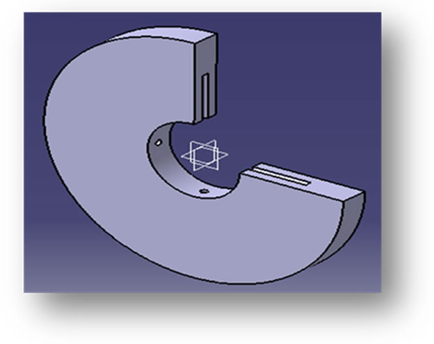
Figure 4. Cut section of special purpose die.
facilitates study of friction and wear characteristics in sliding contact under desired conditions. Sliding occurs between the stationary pin and a rotating disc. Normal load, rotational speed and wear track diameter can be varied to suit the test conditions. Tangential frictional force and wear are monitored with electronic sensors and recorded on computer .These parameters are available as function of load and speed. Reading of wear are taken after making all the necessary connections and Sliding speed is calculated as follows Sliding speed = π × D × N/60,000.
Cross section Area of rod = π × d2/4 where, D = Diameter of wear track in mm. N = Disc speed in rpm. T = Test duration in sec, d = diameter of specimen rod.
3.1. Calculation of Constants [5,6]
Let, W = Wear in micron, L = Load in N, V = Sliding Speed in m/s, T = Test duration in sec.
K = Proportionality Constant, a, b, & c are the index of load, speed & time respectively,W1 and W2 are wears corresponding to loads L1, L2; Sliding speeds V1, V2 and testing time T1, T2
Equation of wear is –W = K × La × Vb × Tc
3.1.1. Calculation of “a”
Table 1 shows Calculation of “a” by considering V & T Constant i.e. (k × Vb × Tc = Cont).
W1/W2 = (L1/L2)a
ln(W1/W2) =a × ln(L1/L2)
a = ln(W1/W2)/ln(L1/L2)
Regression Analysis: WEAR versus LOAD
The regression equation is
WEAR = –1.77 + 0.437 LOAD
Predictor Coef SE Coef T P VIF
Constant –1.7670 0.6073 –2.91 0.101
LOAD 0.43750 0.01685 25.97 0.001 1.000
S = 0.370355 R-Sq = 99.7% R-Sq(adj) = 99.6%
3.1.2. Calculation of “b”
Similarly, b is
b= ln (W1/W2) / ln(V1/V2)
where, k × La × Tc = Constant
Table 2 shows calculations of b by considering L &T constant.
Regression Analysis: WEAR versus SLIDING SPEED
The regression equation is
WEAR = –52.0 + 33.4 SLIDING SPEED
Predictor Coef SE Coef T P VIF
Constant –52.0010 0.0022 –23758.06 0.000
SLIDING SPEED 33.4093 0.0005 73904.47 0.000 1.000
S = 0.000423587 R-Sq = 100.0% R-Sq(adj) = 100.0%
3.1.3. Calculations of “c”
c = ln (W1/W2)/ln (T1/T2) where k × La × Vb = Constant.
Table 3 shows calculations of “c” by considering L & V Constant.
Regression Analysis: WEAR versus TEST TIME
The regression equation is
WEAR = 11.5 + 0.0800 TEST TIME
Predictor Coef SE Coef T P
Constant 11.5000 0.8660 13.28 0.006
TEST TIME 0.080000 0.003162 25.30 0.002
S = 0.707107 R-Sq = 99.7% R-Sq(adj) = 99.5%
3.1.4. Calculations of “k”
Table 4 shows calculations of “k”.