Understanding the Theory of Karp, Miller and Winograd

Athanasios I. Margaris

Department of Digital Systems, Gaiopolis Campus, University of Thessaly, Larissa, Greece.

DOI: 10.4236/jamp.2024.124075                

Abstract

The objective of this tutorial is to present the fundamental theory of Karp, Miller and Winograd, whose seminal paper laid the foundations regarding the systematic description of the organization of computations in systems of uniform recurrent equations by means of graph structures, via the definition of computability conditions and techniques for the construction of one-dimensional and multi-dimensional scheduling functions. Besides the description of this theory, the paper presents improvements and revisions made by other authors and furthermore, points out the differences regarding the conditions of causality and dependency between the general case of systems of recurrent equations and the special case of multiple nested loops.

Keywords

Computability, Scheduling, Computations, Recurrent Equations

1. Introduction

A very important topic in the field of all mathematical sciences is closely related to the organization of computations associated with uniform recurrent equations, namely, recurrent equations characterized by the presence of uniform data dependencies. This problem was first formulated and studied in 1967 by Karp, Miller and Winograd (KMW) [1] , via the development of an appropriate model describing the organization of those computations, as well as the inherent parallelism involved in the solution of this type of systems. This model is capable to describe a wide range of algorithms and applications from the field of mathematics and computer science, and to provide an accurate description of such an organization [2] . Although the model of Karp, Miller and Winograd, which was created in an attempt to study explicit schemes of difference equations, is purely theoretical, its conclusions were extended and clarified by later works, and the number of its applications was so large, that this work is considered one of the most important in the field. For example, the well-known Lamport’s method of hyperplanes [3] , as well as the methodology of spatio-temporal mappings [4] [5] , related to the field of automatic parallelization of nested loops, are strongly based on the model of KMW. Furthermore, the nested loop parallelization algorithm of Allen and Kennedy [6] has its roots in this model, since it can be seen as a special case of the graph decomposition procedure of Karp, Miller and Winograd.

To understand the necessity to formalize the organization of calculations, let us consider the Laplace differential equation as an example [7] :

$\frac{{\partial }^{2}T}{\partial x^2}+\frac{{\partial }^{2}T}{\partial y^2}=f\left(x\mathrm{,}y\right)$

that describes the distribution $T\left(x\mathrm{,}y\right)$ of the temperature at each point $\left(x\mathrm{,}y\right)$ on the surface of a thin square plate of thickness $\Delta z$ (much smaller than the dimensions of the plate). The plate is considered insulated in such a way, that heat flows only along the x and y directions. If there are no sources or sinks of heat, described by the function $f\left(x\mathrm{,}y\right)$ , the Laplace equation becomes a homogenous one. The equation is constructed by relying on physical arguments, while its numerical solution relies on the application of the well-known finite difference method. This method is based on the definition of a grid of points or nodes on the surface of the heated plate and on the numerical calculation of the temperature, at each point or node of this grid. Even though this example concerns a scalar function, such as the temperature, the same procedure can be used for the numerical solution of partial differential equations associated with vector functions, such as the electric field. The grid used in the finite difference method is usually defined in Cartesian coordinates, although in general it can be defined in any system of rectangular or curvilinear coordinates, according to the geometry of the problem and the way of the definition of the boundary conditions. The estimation of the temperature at each node of the grid allows us to determine the values of the temperature at any other point, resorting to methods such as interpolation, extrapolation or function approximation. Note, that in order to obtain a complete solution to the problem, it is also necessary to define the appropriate boundary conditions, which consist of setting constant temperature values for each of the four edges of the square plate. Based on all the above, we find that the finite difference method is nothing more than the discretization of a partial differential equation, both in space and in time, a process that leads to the construction of the corresponding difference equation.

In order to apply the above procedure to the Laplace equation, we have to define the appropriate grid structure (see Figure 1(a)) and then replace the partial derivatives ${\partial }^{2}T/\partial x^2$ and ${\partial }^{2}T/\partial y^2$ with the corresponding central differences as:

$\frac{{\partial }^{2}T}{\partial x^2}=\frac{T_{i+\mathrm{1,}j}-2T_{i\mathrm{,}j}+T_{i-\mathrm{1,}j}}{\Delta x^2}$

Figure 1. (a) The grid defined on the surface of a square heated plate for the numerical solution of Laplace’s equation by the finite difference method; (b) The grid nodes that identify the spatial points of the calculation of the temperature function $T\left(x\mathrm{,}y\right)$ , together with their coordinates (Source: Chapra & Canale, Figs. 29.2 and 29.3).

$\frac{{\partial }^{2}T}{\partial y^2}=\frac{T_{i\mathrm{,}j+1}-2T_{i\mathrm{,}j}+T_{i\mathrm{,}j-1}}{\Delta y^2}$

with errors $O\left[\Delta {\left(x\right)}^2\right]$ and $O\left[\Delta {\left(y\right)}^2\right]$ , respectively. In this case, the Laplace’s equation gets the form:

$\frac{T_{i+\mathrm{1,}j}-2T_{i\mathrm{,}j}+T_{i-\mathrm{1,}j}}{\Delta x^2}+\frac{T_{i\mathrm{,}j+1}-2T_{i\mathrm{,}j}+T_{i\mathrm{,}j-1}}{\Delta y^2}=0$

and for the special case of the square plate, the above relation becomes:

$T_{i+\mathrm{1,}j}+T_{i-\mathrm{1,}j}+T_{i\mathrm{,}j+1}+T_{i\mathrm{,}j-1}-4T_{i\mathrm{,}j}=0$

where we have set $\Delta x=\Delta y=h$ . The above expression, known as the Laplace’s difference equation, is valid for all the interior points of the plate. Therefore, if the appropriate boundary conditions (such as Dirichlet’s conditions) are defined, then, it is possible to calculate the temperature value at each of the nodes of the grid defined on the surface of the plate, such as the nine points depicted in Figure 1(b). The outcome of this procedure is a system of difference equations or recurrent equations, whose number is equal to the number of grid nodes, or equivalently, to the number of functions to be computed. The work of KMW is concerned with the organization of computations associated with each of those grid nodes, as well as the description of the related concepts and techniques, such as the notion of computability and scheduling functions.

2. Defining the Basic Concepts

Returning to the presentation of the theory of KMW, it deals with the study of a system of uniform recurrent equations, each one having the form:

${\alpha }_i\left(p\right)=f_i\left({\alpha }_i\left(p-d_{i1}\right)\mathrm{,}{\alpha }_i\left(p-d_{i2}\right)\mathrm{,}\cdots \mathrm{,}{\alpha }_i\left(p-d_{im}\right)\right)$

$\left(1\le i\le n\right)$ , with the functions ${\alpha }_i\left(p\right)$ to represent matrix-type variables. The values of these variables must be computed in the grid points described by the integer vectors $p$ , used as arguments to the above functions. These vectors are known as iteration vectors, with this name being justified by the fact, that the described procedure is an iterative process, in the sense that the computation of the above variables is performed in an iterative way at the positions of all integer points that are supposed to define a subset R of the space ${\mathbb{Z}}^n$ , which is known as the iteration space, or, equivalently, as the computational domain. From this viewpoint, the boundary values, defined in the previous example (if required), are defined as integer points that do not belong to the set R. On the other hand, the vectors $d_{ij}$ $\left(1\le i\le n\mathrm{,}1\le j\le m\right)$ appearing in the above equations are known as dependence vectors, while the functions $f_i\left(x_1\mathrm{,}{x}_2\mathrm{,}\cdots \mathrm{,}{x}_m\right)$ $\left(1\le i\le n\right)$ , are strictly dependent on each of their arguments, meaning that whatever value $c_j$ is assigned to the variable $x_j$ $\left(j_{n}eqi\right)$ , the value of the function $f_i\left(c_1\mathrm{,}{c}_2\mathrm{,}\cdots \mathrm{,}{c}_{i-1}\mathrm{,}{x}_i\mathrm{,}{c}_{i+1}\mathrm{,}\cdots \mathrm{,}{b}_s\right)$ is not a constant. Note, that the number of arguments (namely, the value of m) in these functions, is generally different for each one of them, and since we are only interested in the organization of computations and not in the exact process performed by them, the nature, as well as the number of definitions of the functions $f_i$ $\left(1\le i\le n\right)$ , is completely ignored.

A basic requirement for the computation of the function ${\alpha }_i\left(p\right)$ at the position $p$ of the iteration space, is the availability at the time of computation, of the complete set of the values of the functions ${\alpha }_i\left(p-d_{i1}\right)\mathrm{,}{\alpha }_i\left(p-d_{i2}\right)\mathrm{,}\cdots \mathrm{,}{\alpha }_i\left(p-d_{im}\right)$ $\left(1\le i\le n\right)$ , which should already be calculated and known in advance, meaning that there is a dependence between the value ${\alpha }_i\left(p\right)$ and each one of the above values. The theory of KMW deals with systems of recurrent equations characterized by uniform dependencies, described by the well-known dependence diagrams, namely, by directed graphs $G=\left(V\mathrm{,}E\right)$ of finite size, defined in the region of interest $R\subset {\mathbb{Z}}^n$ . In these graphs, the sets of vertices V and edges E, are defined as finite sets of the form $V=\left\{{\upsilon }_1\mathrm{,}{\upsilon }_2\mathrm{,}\cdots \mathrm{,}{\upsilon }_m\right\}$ and $E\mathrm{<mo>\; =\; </mo>\; <mo>\; \{\; </mo>}{e}_1\mathrm{,}{e}_2\mathrm{,}\cdots \mathrm{,}{e}_{ell}\mathrm{<mo>\; \}\; </mo>}$ , respectivelly. The vertex set of such a graph has the form of a Cartesian product $\left\{\mathrm{1,2,}\cdots \mathrm{,}m\right\}\times P$ . The graph contains an edge from vertex $\left(j\mathrm{,}q\right)$ to vertex $\left(i\mathrm{,}p\right)$ , if the value of the function ${\alpha }_i\left(p\right)$ depends on the value of the function ${\alpha }_j\left(q\right)$ , with the label of this edge to be an appropriate dependence vector, which is a vector of integers (and in the general case, a polyhedron). On the other hand, each vertex of such a graph represents the complete set of the computations associated with the instances of the same variable to be computed. Note, that such a graph can have one or more loops, namely, edges whose source and destination are the same vertex, as well as one or more cycles, namely closed paths that start and end at the same vertex as before, but they pass also through other vertices. In the general case, the label associated with a vertex v in such a graph, is a polyhedron $P_v$ , which belongs to the set ${\mathbb{Q}}^{d_v}$ where $d_v$ is the dimension of the iteration space of vertex v, while, the label associated with an edge joining two vertices v and y, is a polyhedron defined in the space ${\mathbb{Q}}^{d_v+d_y}$ . Note, that the dimension of the vertex iteration space for the special case of a nested iterative loop is equal to the number of loops of the nested structure enclosing the statement associated with this vertex. This type of graph for the general case of systems of recurrent equations is known as Generalized Dependence Graph (GDG), in the sense that it contains as many vertices as iteration vectors. A simplified version of such a graph that used in the automatic parallelization of multiple nested loops is known as Expanded Dependence Graph (EDG).

Denoting by $e_{11}\mathrm{,}{e}_{12}\mathrm{,}\cdots \mathrm{,}{e}_{1k}$ the edges of the graph G starting from vertex ${\upsilon }_i$ and ending at vertices ${\upsilon }_{i1}\mathrm{,}{\upsilon }_{i2}\mathrm{,}\cdots \mathrm{,}{\upsilon }_{ik}$ respectively, and by $d_{ij}$ the weight vector of length n associated with the edge $e_{ij}$ , the equation corresponding to the vertex ${\upsilon }_i$ will have the form:

${\alpha }_i\left(p\right)=f_i\left({\alpha }_{i1}\left(p-d_{i1}\right)\mathrm{,}{\alpha }_{i2}\left(p-d_{i2}\right)\mathrm{,}\cdots \mathrm{,}{\alpha }_{ik}\left(p-d_{ik}\right)\right)$

It is not difficult to see, that if we know the mathematical form of a system of uniform recurrent equations, we can easily construct the associated dependence graph, and vice versa, meaning that these two forms of describing the system are in fact, equivalent descriptions of the system under consideration.

3. Computability and Scheduling of Calculations

From the above description, it is clear that there are two main issues associated with the computations in systems of uniform recurrent equations, namely, 1) the issue of computability and 2) the issue of scheduling. In particular, the computability problem, attempts to give an answer to the question whether the recurrent process described above, is associated with computable functions ${\alpha }_k\left(p\right)$ , or not. If it turns out that the functions under consideration are computable functions, then the problem of scheduling emerges, associated with the construction of a scheduling function that determines the moment of execution for each one of the involved computations. A key assumption commonly used in such calculations is the availability of an infinite number of processors in the underlying parallel system, so that, in each case, as many processors as needed, are available. Even though this requirement, will never be met in practice, the scheduling function defined in this way, eventually allows the mapping of the computations to a finite number of processors.

Why it is necessary to define such a scheduling function? This necessity stems from the fact, that the algebraic structure describing the iteration space does not contain any information regarding the order in which the involved computations should be performed and therefore, this execution order should be specified separately. It turns out, that each one of these two problems (namely, computability and scheduling), is the dual of the other (as dualism is defined in the field of linear programming). These problems are closely related to the fact that the computation of the functions that appear in the left-hand size of the recurrent equations requires the computation and the availability of the values of the complete set of quantities used as arguments to those functions, which, in turn requires the values of their own arguments, and so on. Regarding the question of calculating all those values, there are two possibilities which may arise in practice, depending on the nature of the dependencies defined between these functions: either the calculation of all these values will take place in a finite period of time, or the dependencies are such that, the waiting period for the availability of a value used as an argument to a function has an infinite value, in which case, the recurrent procedure is characterised as non-computable. A typical example of a non-computable process is a circular wait situation, in which each one of two function values is waiting for the other value to become available, a situation which is very common in operating systems and it is described by the term deadlock [8] .

As Feautrier [9] points out that the concepts of scheduling and the associated tables have their roots in Operations Research and in PERT diagrams [10] . However, the scheduling tables cannot be used in the field of parallel processing, in the way used in Operations Research, since there are several practical difficulties: the grouping of elementary computations into tasks, is not a trivial process, and generally speaking, it is difficult or impossible to know in advance, the execution time instance as well as the total execution time of each task. To overcome these difficulties, only a very small number of elementary computations can be assigned to each task. In the extreme case, each task is associated with a single statement, and since in this case, the number of processes involved, is very large, we can resort only to an asymptotic analysis of the situation. In this type of analysis, the knowledge of the exact execution time is not so important and therefore, it is common practice to assign to each execution time interval, a value of unity. Furthermore, the inability to construct scheduling tables makes it as the only possibility, the expression of the involved functions in closed form.

The problem of scheduling is one of the fundamental problems associated with the automatic parallelization of nested loops, and it can be handled by resorting to a special class of scheduling functions, and more specifically, to linear scheduling functions, that do not apply to all systems of uniform recurrent equations. These functions are constructed via the application of the well-known method of hyperplanes [3] that transforms a traditional sequential nested loop of depth $d=n$ , into a parallel loop, consisting of an outer sequential loop and $n-1$ inner parallel loops. There are several types of linear scheduling functions, with the most general and commonly used type, being the affine linear functions, used initially in systolic array design [11] [12] from systems of recurrent equations. These functions, are defined as mappings $V\times {\mathbb{Z}}^n\mapsto \mathbb{Q}$ of the form $S\left(\upsilon \mathrm{,}p\right)={\Pi }_{\upsilon }\cdot p+{\rho }_{\upsilon }$ (or of the form $S\left(\upsilon \mathrm{,}p\right)=\lfloor {\Pi }_{\upsilon }\cdot p+{\rho }_{\upsilon }\rfloor$ if the mapping S is defined as $S\mathrm{<mo>\; :\; </mo>}V\times {\mathbb{Z}}^n\mapsto \mathbb{N}$ —in this case, they are characterized as semi-linear or nearly linear) where ${\Pi }_{\upsilon }\in {\mathbb{Q}}^n$ is the so-called scheduling vector, selected such that ${\Pi }_{\upsilon }D\ge 1$ where $D$ is the dependence matrix (or equivalently ${\Pi }_{\upsilon }{d}_i\ge 1$ for each dependence vector $d_i\in D$ ), a condition that guarantees the preservation of the underlying data dependencies and allows the characterization of the scheduling function as a valid scheduling function, and ${\rho }_{\upsilon }\in \mathbb{Q}$ a parameter with a value of ${\rho }_{\upsilon }=-\min \left\{{\Pi }_{\upsilon }\cdot p\mathrm{,}p\in R\right\}$ (this conditions allows the execution of the calculations to start at time $t=0$ ). The use of the subscript $\upsilon$ in this notation, indicates that the quantities ${\Pi }_{\upsilon }$ and ${\rho }_{\upsilon }$ , in general, they have different values for each vertex ${\upsilon }_k$ , namely, for each calculation ${\alpha }_k\left(p\right)$ , while the dependence matrix $D$ , contains as columns the dependence vectors. In the special case, in which the vector ${\Pi }_{\upsilon }$ has the same value for all vertices, then the affine scheduling function is characterized as a shifted linear scheduling function (due to the non-zero value of the parameter ${\rho }_{\upsilon }$ ), and furthermore, if the condition ${\rho }_{\upsilon }=0$ holds, then we simply refer to a linear scheduling function. Note, that even though the calculation of the vector ${\Pi }_{\upsilon }$ and the parameter ${\rho }_{\upsilon }$ can be performed by constructing and solving, via linear programming techniques, an appropriate system of equations that contains one equation for each grid point $p$ , however, in practice, due to the very large number of equations, the determination of these functions in closed form, is carried out by other methods. These types of scheduling functions are particularly popular, and they are widely used in almost all cases of scientific applications, because they allow the automatic code generation for the parallel nested loops, with only a small overhead.

In order to give a mathematical description, let us define a precedence relation, described by means of a precedence graph, as a relation between two computations that determines which one of them will be executed first, or equivalently, specifies the order in which the evaluation of the functions ${\alpha }_i\left(p\right)$ at the different grid points $p$ will take place. Let us consider an ordered pair $\left(k\mathrm{,}p\right)$ of the set $\left\{\mathrm{1,2,3,}\cdots \mathrm{,}m\right\}\times P$ , with the first element k to be an integer in the interval $1\le k\le m$ and the second element $p$ to be a vector of n elements, that identifies the function ${\alpha }_k\left(p\right)$ to be computed. In this case, the pair $\left(k\mathrm{,}p\right)$ depends directly on the pair $\left(\mathcal{l}\mathrm{,}q\right)$ , or, in a symbolic notation, $\left(k\mathrm{,}p\right)\stackrel{1}{\to }\left(\mathcal{l}\mathrm{,}q\right)$ , if and only if a) $p\in P$ and b) the precedence graph that describes the problem, contains an edge directed from vertex ${\upsilon }_k$ to vertex ${\upsilon }_{\mathcal{l}}$ such that $p-d_k=q$ , for some dependence vector $d_k$ . In other words, the condition $\left(k\mathrm{,}p\right)\stackrel{1}{\to }\left(\mathcal{l}\mathrm{,}q\right)$ holds, if and only if the function ${\alpha }_{\mathcal{l}}\left(q\right)$ is one of the arguments of the function ${\alpha }_k\left(p\right)$ . The subscript 1 used in this notation indicates that the dependence between the pairs $\left(k\mathrm{,}p\right)$ and $\left(\mathcal{l}\mathrm{,}q\right)$ is a direct dependence between these two pairs, rather than an indirect one. Note, that if the pairs $\left(k\mathrm{,}p\right)$ and $\left(\mathcal{l}\mathrm{,}q\right)$ are identical, meaning that if $k=\mathcal{l}$ and $p=q$ , we simply write $\left(k\mathrm{,}p\right)\stackrel{0}{\to }\left(\mathcal{l}\mathrm{,}q\right)$ , while in the general case of a t-dependence, it is defined inductively in the following way: we write $\left(k\mathrm{,}p\right)\stackrel{t}{\to }\left(\mathcal{l}\mathrm{,}q\right)$ if there exists a pair $\left(h\mathrm{,}r\right)$ such that $\left(k\mathrm{,}p\right)\stackrel{t-1}{\to }\left(h\mathrm{,}r\right)$ and $\left(h\mathrm{,}r\right)\stackrel{1}{\to }\left(\mathcal{l}\mathrm{,}q\right)$ , and with the basic step of this inductive process, being the condition $\left(k\mathrm{,}p\right)\stackrel{0}{\to }\left(\mathcal{l}\mathrm{,}q\right)$ defined earlier. If for some positive integer t, it holds that $\left(k\mathrm{,}p\right)\stackrel{t}{\to }\left(\mathcal{l}\mathrm{,}q\right)$ , then, we simply write $\left(k\mathrm{,}p\right)\to \left(\mathcal{l}\mathrm{,}q\right)$ . The meaning of this last expression, is that the value of the function ${\alpha }_{\mathcal{l}}\left(q\right)$ should be computed before the value of the function ${\alpha }_k\left(p\right)$ , a condition that is the fundamental property of every valid scheduling function.

4. One- and Multi-Dimensional Scheduling

According to the description given so far, the scheduling of a generic computation process, is defined as a function of the form $S\mathrm{<mo>\; :\; </mo>}\left\{\mathrm{1,2,}\cdots \mathrm{,}m\right\}\times R\mapsto {\mathbb{Z}}^{+}$ , that takes as input an ordered pair $\left(k\mathrm{,}p\right)$ describing the computation of the function ${\alpha }_k\left(p\right)$ and returns the execution time instance $S\left(k\mathrm{,}p\right)$ of this computation. In order such a function to be valid, the following condition must be satisfied: if $\left(k\mathrm{,}p\right)\to \left(\mathcal{l}\mathrm{,}q\right)$ , then $S\left(k\mathrm{,}p\right)>S\left(\mathcal{l}\mathrm{,}q\right)$ . This condition stems from the fact that the dependencies between calculations must be preserved under the application of the scheduling function. In other words, as long as the value ${\alpha }_k\left(p\right)$ depends on the value ${\alpha }_{\mathcal{l}}\left(q\right)$ (in the sense that the latter value must be known and available at the estimation time of the first value), it must be calculated afterwards. Therefore, the condition $S\left(k\mathrm{,}p\right)>S\left(\mathcal{l}\mathrm{,}q\right)$ must be hold. If we make the assumption that the duration of each computation is equal to unity (this assumption allows us to describe the duration of the execution of each computation, as lengths of paths defined on the precedence graph), the above relation is alternatively formulated as $S\left(k\mathrm{,}p\right)\ge S\left(\mathcal{l}\mathrm{,}q\right)+1$ . Therefore, the start time $S\left(k\mathrm{,}p\right)$ of the computation ${\alpha }_k\left(p\right)$ must be greater than or equal to the completion time of the computation ${\alpha }_{\mathcal{l}}\left(q\right)$ , which in turn, is equal to the start time $S\left(\mathcal{l}\mathrm{,}q\right)$ of the computation ${\alpha }_{\mathcal{l}}\left(q\right)$ plus the time duration of this calculation (which is equal to one). The above requirement expresses a condition of causality, which in turn is imposed by the necessity of maintaining the existing dependencies between the computations.

The scheduling function defined above, is associated with the so-called one-dimensional scheduling, in the sense that the execution time instance of the computation performed at the grid point $p$ , is described by a simple positive integer value. However, multi-dimensional scheduling functions can also defined, as mappings in the form $S\mathrm{<mo>\; :\; </mo>}V\times R\mapsto {\mathbb{Z}}^{+}{}^d$ . Using these special mappings, it is possible to define logical execution time instances, that are not described by a simple number, but instead, by a vector of d values which can be interpreted in the same way as a date, meaning, that the most significant of these values represents days, while the remaining values represent, respectively, hours, minutes, seconds, etc. This type of scheduling is applied in more complex cases for which the construction of an affine one-dimensional scheduling function is not possible. Of course, since in this case, the execution time instance is not a simple number but a whole tuple of d elements, an ordering relation has to be defined, allowing the characterization of such a tuple as smaller (earlier) or larger (later) than another one. In practice, for this purpose, the well-known lexicographic ordering is a common choice. This ordering is used very frequently in mathematics and computer science and a well-known example of its use, is the ordering of the iterations of a multiple nested loop. If we denote this lexicographic ordering by the symbol $\gg$ , a multi-dimensional scheduling function is characterized as a valid one, if it satisfies the condition $\left(k\mathrm{,}p\right)\to \left(\mathcal{l}\mathrm{,}q\right)\Rightarrow S\left(k\mathrm{,}p\right)\gg S\left(\mathcal{l}\mathrm{,}q\right)$ . This condition is exactly the same as the one we used to characterize a valid one-dimensional scheduling function, except that the relevant quantities appearing are tuples of d elements. Assuming again that the time duration of the computations is equal to unity, the condition $S\left(k\mathrm{,}p\right)\ge S\left(\mathcal{l}\mathrm{,}q\right)+1$ for the multi-dimensional scheduling, is formulated as $\exists k\mathrm{,}1\le k\le d$ : s.t $\forall i:i<k$ ,

${\left[S\left(k\mathrm{,}p\right)\right]}_i={\left[S\left(\mathcal{l}\mathrm{,}q\right)\right]}_i\text{and}{\left[S\left(k\mathrm{,}p\right)\right]}_k\le {\left[S\left(\mathcal{l}\mathrm{,}q\right)\right]}_k+1$

In the above expression, the use of the operator [...] stems from the fact that the range of the associated mapping, is the set $\mathbb{Q}$ of rational numbers. As in the case of one-dimensional scheduling, the affine multi-dimensional scheduling is defined as a mapping of the form $S\mathrm{<mo>\; :\; </mo>}V\times {\mathbb{Z}}^n\mapsto {\mathbb{Q}}^n$ such that:

$\left(k\mathrm{,}p\right)\mapsto \left(x_{\upsilon }^1\cdot p+{\rho }_{\upsilon }^1\mathrm{,}{x}_{\upsilon }^2\cdot p+{\rho }_{\upsilon }^2\mathrm{,}\cdots \mathrm{,}{x}_{\upsilon }^d\cdot p+{\rho }_{\upsilon }^d\right)$

In the above expression, the vectors $x_{\upsilon }^i$ $\left(1\le i\le d\right)$ are all different from each other. If $x_{\upsilon }^1=x_{\upsilon }^2=\cdots =x_{\upsilon }^d$ , then, the above condition for each edge $e\in E$ of the graph takes the form:

$\forall e\in E\mathrm{,}\exists k_e\mathrm{<mo>\; :\; </mo>1}\le k_e\le d\mathrm{<mo>\; :\; </mo>,}\forall i\mathrm{<mo>\; :\; </mo>1}\le i\le k_e$

$\{\begin{array}{l}{x}^i\cdot w\left(e\right)+{\rho }_{x_e}^i-{\rho }_{y_e}^i=0\\ x^{k_e}\cdot w\left(e\right)+{\rho }_{x_e}^{k_e}-{\rho }_{y_e}^{k_e}\ge 1\end{array}$

with the subscripts $x_e$ and $y_e$ describing the vertices of the graph associated with the edge e (starting at vertex $x_e$ and ending at vertex $y_e$ ), and the subscript $\upsilon$ denoting the vertex of the graph associated with the computation to be scheduled. The equations $x^{k_e}\cdot w\left(e\right)+{\rho }_{x_e}^{k_e}-{\rho }_{y_e}^{k_e}\ge 1$ and $x^i\cdot w\left(e\right)+{\rho }_{x_e}^i-{\rho }_{y_e}^i=0$ appearing in the above condition, are hyperplane equations, defining a strongly separating and a weakly separating hyperplane, respectively.

The problem of determining affine scheduling functions for both the one-dimensional and the multi-dimensional case is described by Feautrier [9] [13] in its most general form, which does not refer to a particular dependency graph, but to a (potentially) infinite family of such graphs, each member of this family being determined by one or more integer parameters which together constitute the parameter vector $n$ . Consequently, the affine scheduling function does not have the simple form $S\left(\upsilon \mathrm{,}p\right)=X_{\upsilon }\cdot p+{\rho }_{\upsilon }$ but the more general form:

$S\left(\upsilon \mathrm{,}p\right)={\Pi }_{\upsilon }\cdot p+s_{\upsilon }\cdot n+{\rho }_{\upsilon }$

where ${\Pi }_{\upsilon }$ and $s_{\upsilon }$ are unknown vectors with fixed rational coordinates and ${\rho }_{\upsilon }$ is an unknown constant. It is not difficult to realize, that the problem of determining the scheduling function is related to the estimation of the above unknown parameters, in such a way that the causality condition is still satisfied, and to the selection of a solution that leads to the optimization of the value of the appropriate performance parameter, such as the minimum time delay. The form of the above equation is documented by the fact that the solution of the scheduling problem for increasingly larger values of n, leads to functions which in the limit of large values of $n$ , are linear with respect to $n$ [14] . The above general equation can be considered as a type of template that every scheduling function should follow, and in the literature can be found simpler expressions, that use, for example, the same vector ${\Pi }_{\upsilon }$ for all vertices of the graph (as in the case of uniform recurrent equations) with the resulting function, in this case, to be known as the wavefront.

5. Solving the Scheduling Problem

A straightforward way to determine the unknown parameters ${\Pi }_{\upsilon }$ , $s_{\upsilon }$ and ${\rho }_{\upsilon }$ , appearing in the linear scheduling functions, is to substitute in the condition $S\left(y_e\mathrm{,}y\right)\ge S\left(x_e\mathrm{,}x\right)+1$ for each edge e of the graph, starting at vertex $x_e$ and ending at vertex $y_e$ , the appropriate values of the parameters x, y and $n$ and then solve the resulting system of linear inequalities by resorting to classical linear programming methods, such as the simplex method. However, the number of inequalities emerging in this way, can be very large (theoretically infinite), and furthermore, there is absolutely no guarantee, that in these inequalities, all important constraints have been included. Therefore, this technique is in fact, not applicable. Feautrier describes two basic methods for solving this problem, and more specifically, the vertex method [9] , as well as another method based on the so-called affine form of Farkas’ lemma [15] . Of these two methods, the vertex method is based on the observation that a polyhedron can be described either as a set of points satisfying a finite set of linear inequalities, or as the convex hull of a set of points and consists of: a) the determination of the generating system for all polyhedra $D_{\upsilon }$ where $\upsilon \in V$ and $e\in E$ , b) the construction of the inequality $S\left(y_e\mathrm{,}y\right)\ge S\left(x_e\mathrm{,}x\right)+1$ for all vertices of the polyhedron $R_e$ associated with edge e, as well as the inequality $S\left(\upsilon \mathrm{,}x\right)\ge 0$ for all vertices of $D_{\upsilon }$ and c) the solution of the finite system of linear inequalities obtained in the above way, using algorithms such as Chernikova’s algorithm [16] .

The above method, which allows the transformation of a set of inequalities, into a set of polyhedral vertices, has very high computational cost and therefore, a simpler method is required that does not based on new transformations, but on the original inequalities. Such a method relies on the affine form of Farkas’ lemma, formulated in the following way: let D be a non-empty polyhedron, defined by p affine inequalities of the form $a_{k}x+b_k\ge 0$ $\left(1\le k\le p\right)$ . In this case, an affine form $\psi$ is nonnegative anywhere in D, if and only if it is a positive affine combination of the form:

$\psi \left(x\right)={\lambda }_0+{\displaystyle \underset{k}{\sum }}{\lambda }_k\left(a_{k}x+b_k\right)\mathrm{,}{\lambda }_k\ge 0$

This method relies on the observation that an affine scheduling function $S\left(\upsilon \mathrm{,}p\right)=X_{\upsilon }\cdot p+s_{\upsilon }\cdot n+{\rho }_{\upsilon }$ takes non-negative values if and only if there are Farkas multipliers ${\mu }_{S_k}$ such that:

$S\left(\upsilon \mathrm{,}p\right)={\mu }_{S_0}+{\displaystyle \underset{k=1}{\overset{m_S}{\sum }}}{\mu }_{S_k}\underset{A}{\underset{︸}{\left(a_{S_k}\left(\begin{array}{c}x\\ n\end{array}\right)+b_{S_k}\right)}}$

where $m_S$ is the set of inequalities of D, with each of the expressions A, whose values are greater than or equal to zero, being the inequalities defining each polyhedron $D_{\upsilon }$ . The above equation is a new representation of the original expression, and can be used in its place, in all relevant calculations. Consequently, if numerical values for the Farkas coefficients ${\mu }_{S_k}$ are determined, then, we can immediately construct the appropriate version of the original expression.

The calculation of Farkas multipliers, is based on the observation that for an affine scheduling function $S\left(\upsilon \mathrm{,}p\right)$ , the time delay associated with each edge $e\in E$ of the graph, is given by the expression:

${\Delta }_e=S\left(y_e\mathrm{,}y\right)-S\left(x_e\mathrm{,}x\right)-1$

where $x_e$ and $y_e$ are the source and destination of edge e of graph G, respectively. Therefore, there will be Farkas multipliers such that:

$S\left(y_e\mathrm{,}y\right)-S\left(x_e\mathrm{,}x-1\right)={\lambda }_{e_0}+{\displaystyle \underset{k=1}{\overset{m_S}{\sum }}}{\lambda }_{e_k}\underset{B}{\underset{︸}{\left(c_{e_k}\left(\begin{array}{c}x\\ y\\ n\end{array}\right)+d_{e_k}\right)}}$

In the above equation, the expressions denoted by B (whose values are also greater than or equal to zero), define the polyhedron of dependencies of edge e. The final result of this procedure is a system of linear equations with unknown Farkas multipliers, with positive values. Having calculated these coefficients, we can then determine the required scheduling function. As Feautrier points out, using a technique similar to Gauss-Jordan elimination, we can significantly reduce the size of the problem and make the algorithm even more efficient.

6. Selecting the Optimal Time Routing Function

The number of valid scheduling functions is obviously not countable, and therefore, the most appropriate function for each case has to be identified, in the simplest possible way. When all the iteration spaces are finite and there is at least one affine scheduling function, it can be proven that there is at least one affine form $L=h\cdot n+k$ such that, for every $\upsilon \in V$ and for every $x\in D_{\upsilon }$ , the condition $L-S\left(\upsilon \mathrm{,}x\right)\ge 0$ holds. If we take into account that the latency increases with the components of the vector $n$ , the components of the vector $h$ will be positive numbers, and resorting to Farkas’ lemma, we can write:

$L-S\left(\upsilon \mathrm{,}x\right)={\nu }_{S_0}+{\displaystyle \underset{k=1}{\overset{m_S}{\sum }}}{\nu }_{S_k}\left(a_{S_k}\left(\begin{array}{c}x\\ n\end{array}\right)+b_{S_k}\right)$

We are now able to compute the values of the coefficients ${\nu }_{S_k}$ , which lead to an affine scheduling function, characterized by the minimum time lag. Alternatively, we can estimate a scheduling function whose latency is characterized by an upper bound, namely:

$\left(x\mathrm{,}y\right)\in R_e\iff 1\le S\left(y_e\mathrm{,}y\right)-S\left(x_e\mathrm{,}x\right)\le \delta$

where $\delta$ is a constant term. It turns out that this scheduling function is more restrictive than the functions of this type, that lead to the minimum latency.

Since the above techniques are characterized by a very high sensitivity to the order in which the problem parameters appear in the vector $n$ , it may be difficult to use them in practice. To deal with these situations, an alternative technique devised by Feautrier can be applied, that tries to determine the optimal affine scheduling function via a search procedure, performed in the closure of the set of affine functions under the operation of finding the minimum value. This function has the form $T\left(r\right)=\min S\left(p\right)$ , for all the scheduling functions S that belong to the set of valid affine scheduling functions. The method of Feautrier is based on an ordering relation, defined between the scheduling functions of the form $S_1\prec S_2\equiv \forall p\in R\mathrm{<mo>\; :\; </mo>}{S}_1\left(p\right)\le S_2\left(p\right)$ , as well as to a theorem, according to which, if the functions $S_1$ and $S_2$ satisfy the causality condition for a generalized dependence graph, then the same is true for the function $S_3\left(p\right)=\min \left[S_1\left(p\right)\mathrm{,}{S}_2\left(p\right)\right]$ . Using again the affine form of Farkas’ lemma, a linear program of the form:

$S\left(\upsilon \mathrm{,}x\right)=\min {\mu }_{S_0}+{\displaystyle \underset{k=1}{\overset{m_S}{\sum }}}{\nu }_{S_k}\left(a_{S_k}\left(\begin{array}{c}x\\ n\end{array}\right)+b_{S_k}\right)$

$m\ge 0\mathrm{,}l\ge 0$

$G\left(\begin{array}{c}m\\ l\end{array}\right)\ge 0$

can be formulated, where $\mu$ and $\lambda$ are vectors of Farkas multipliers and with the last condition, to describe some systems of inequality constraints. To ensure that the above procedure leads to a solution expressed in closed form, a parametric solution has to be constructed, whose parameters are functions of $x$ . Applying the duality theorem of linear programming to the linear programs $z=\min \left(kp\right)$ with $m\ge 0$ , $Gp\le h$ and $y=\max \left(ph\right)$ with $nu\ge 0$ , $nuG\le k$ , the construction of the dual of the above program leads to the result:

$S\left(\upsilon \mathrm{,}x\right)=\max n\cdot h\mathrm{,}n\ge 0$

$nG\le \left(\underset{N}{\underset{︸}{\mathrm{0,}\cdots \mathrm{,0}}}\mathrm{,1,}{a}_{S_1}\left(\begin{array}{c}x\\ n\end{array}\right)+b_{S_1}\mathrm{,}\cdots \mathrm{,}{a}_{S_{m_S}}\left(\begin{array}{c}x\\ n\end{array}\right)+b_{S_{m_S}}\mathrm{,}\underset{N^{\prime }}{\underset{︸}{\mathrm{0,0,0,}\cdots \mathrm{,0}}}\right)$

where the parameters N and $N^{\prime }$ are defined as:

$N={\displaystyle \underset{R<S}{\sum }}\left(m_R+1\right)\text{and}{N}^{\prime }={\displaystyle \underset{S<T}{\sum }}\left(m_T+1\right)+|$

To complete the procedure, we need to construct such a problem for each statement S and then to solve each one of these problems in closed form, leading thus to the final solution.

What happens if the complexity of the parallelism is polynomial but not linear, and therefore, there is not an affine scheduling function? In this case, multi-dimensional scheduling functions are constructed, which in a sense, are equivalent to polynomial scheduling. These functions are associated with multiple nested loops, and it interestingly to note, that for any program involving only FOR loops, in which the bounds of the loop counters depend only on program parameters or they are numerical constants or functions of the counters of the outer loops (these programs are known as static control programs), such a multi-dimensional scheduling function can always be constructed. It can also be proven that for each instance of a static control program, a linear scheduling function is always defined. However, a higher dimension for the scheduling process, leads to a lower degree of parallelism. Feautrier [13] presents algorithms for finding such multi-dimensional scheduling functions and also describes the decomposition of scheduling problem into a number of sub-problems related to the strongly connected components of the dependence graph, leading to an algorithm which is a generalization of the loop parallelization algorithm of Allen and Kennedy [6] .

In practice, there are many linear scheduling functions of the form $S\left(\upsilon \mathrm{,}p\right)={\Pi }_{\upsilon }\cdot p+{\rho }_{\upsilon }$ (namely, one function for each vector ${\Pi }_{\upsilon }$ ) and it is quite reasonable to try to identify the optimal one, that leads to the shortest possible execution time. If we take into account that the total execution time has the form:

$\begin{array}{c}{T}_X=1+\max \left\{S\left(\upsilon \mathrm{,}p\right)\mathrm{,}p\in R\right\}\\ =1+\max \left\{\lfloor X_{\upsilon }\cdot p_2\rfloor -\lfloor X_{\upsilon }\cdot p_1\rfloor \right\}\mathrm{,}{p}_1\mathrm{,}{p}_2\in R\end{array}$

where we assume that the calculation starts at $p_1$ and ends at $p_2$ , while the scheduling vector $P$ satisfies the condition $XD\ge 1$ that guarantees the preservation of dependencies, the optimal linear scheduling function, is defined as the function that minimizes the above time. If $T_{\mathcal{l}}$ is this minimum execution time associated with optimal scheduling, then the above definition allows us to write the expression:

$T_{\mathcal{l}}=\min \left\{T_X\mathrm{,}X\in {\mathbb{Q}}^n\mathrm{,}XD\ge 1\right\}$

The problem of identifying the optimal linear scheduling vector for the case of multiple nested loops, has lead to a lot of interesting methods and techniques, such as the method of Shang and Fortes [17] which is based to the partitioning of the solution space containing all the scheduling vectors into convex sub-cones, and to the solution of a linear problem for each sub-cone, in order to identify at compile-time, a subset of vectors that contains the optimal solution.

7. Free Scheduling

One way to evaluate the performance of a scheduling function S, is to count the total number of computations associated with the system of uniform recurrent equations, in the appropriate iteration space and at the time instances determined by the function S. If we assume that each one of these computations is performed in a unit time interval, then this number of computations corresponds to an execution time interval, known as the latency $\mathcal{L}\left(S\mathrm{,}P\right)$ of the scheduling function. It is not difficult to realise, that the duration of this time interval is determine by the completion time of the last computation. In the case of a large number of computations, another quality factor that can be used to describe the situation, is the so-called asymptotic stability [18] , given by the equation:

${\epsilon }_p=\frac{1}{1+\nu P\frac{\mathcal{L}\left(S\mathrm{,}P\right)}{\tau }}$

where P is the number of available processors, $\nu$ is the time duration of the required synchronization processes, and T is the number of points in the iteration space corresponding to the computations to be performed, that can be considered as a measure of the amount of computations. In this case, the ratio $T/\mathcal{L}\left(S\mathrm{,}P\right)$ can be considered as the average degree of parallelism associated with the scheduling function, whose maximum value (corresponding to the scheduling function that leads to the smallest possible latency) is a characteristic of the program being executed.

It is not difficult to see that for a system of uniform recurrent equations, more than one scheduling functions can be defined, each one of them leads to a different number of computations, or in other words, is characterized by its own latency. One such function of particular interest is the so-called free scheduling function. This function corresponds to the case in which, if there is no pair $\left(\mathcal{l}\mathrm{,}q\right)$ such that $q\in R$ and $\left(k\mathrm{,}p\right)\stackrel{1}{\to }\left(\mathcal{l}\mathrm{,}q\right)$ , then the condition $T\left(k\mathrm{,}p\right)=1$ holds, meaning that if there are no dependencies, then the process of calculating the value of the variable ${\alpha }_k\left(p\right)$ will start immediately after the unit time interval of the previous calculation has elapsed. On the other hand, in any other case, this function is defined as:

$T\left(k\mathrm{,}p\right)=1+\max \left\{T\left(\mathcal{l}\mathrm{,}q\right)\mathrm{<mo>\; |\; </mo>}q\in R\text{and}\left(k\mathrm{,}p\right)\stackrel{1}{\to }\left(\mathcal{l}\mathrm{,}q\right)\right\}$

A similar condition can be formulated for the case of the affine one-dimensional scheduling functions. The above relation, as Feautrier comments, is the basis for the inductive methods used to construct scheduling functions. In these methods, we first compute several values of the function $T\left(k\mathrm{,}p\right)$ , based on the above expression. In the next step, using these values, we try to express the scheduling function in closed form, and finally, we check whether the constructed function satisfies the fundamental condition $S\left(k\mathrm{,}p\right)\ge S\left(\mathcal{l}\mathrm{,}q\right)+1$ , as required by any valid scheduling function.

It can be proven, that if a scheduling function can defined, then a unique free scheduling function can also be defined. This function is the fastest scheduling function, in the sense that it defines the earliest possible time at which a computation can be performed. In other words, of all the scheduling functions that can be defined, the free scheduling function is the one that leads to the smallest time latency, but also to the highest degree of parallelism. In a mathematical notation, this condition is formulated as $T\left(k\mathrm{,}p\right)\le S\left(k\mathrm{,}p\right)$ for all pairs $\left(k\mathrm{,}p\right)$ , while, in a verbal description, defines the free scheduling function, as the function that dictates the immediate execution of the associated computation ${\alpha }_k\left(p\right)$ , once the values of all the arguments required to perform this computation, have been computed and they are available. Therefore, it is safe to say, that the free scheduling function, can be considered as a kind of greedy algorithm. In fact, the free scheduling function exists if and only if for every pair $\left(k\mathrm{,}p\right)$ such that $p\in R$ , it is possible to define the function:

$F\left(k\mathrm{,}p\right)=1+\max \left\{t\ge \mathrm{0\; <mo>\; |\; </mo>}\text{exists}\left(\mathcal{l}\mathrm{,}q\right)\mathrm{<mo>\; :\; </mo>}\left(k\mathrm{,}p\right)\stackrel{t}{\to }\left(\mathcal{l}\mathrm{,}q\right)\right\}$

In this case, if there is a free scheduling function, it is simply defined as $T\left(k\mathrm{,}p\right)=F\left(k\mathrm{,}p\right)$ .

In order to generalize this description and define the function $T\left(k\mathrm{,}p\right)$ even when the free scheduling function does not exist, we can very simply write:

$T\left(k\mathrm{,}p\right)=\{\begin{array}{ll}F\left(k\mathrm{,}p\right)\hfill & \text{ifthefunction}F\left(k\mathrm{,}p\right)\hfill \\ \infty \hfill & \text{intheoppositecase}\hfill \end{array}$

In other words, the above definition covers all possible cases, with the condition $T\left(k\mathrm{,}p\right)=F\left(k\mathrm{,}p\right)$ to describe the class of computable functions and the condition $T\left(k\mathrm{,}p\right)=\infty$ to describe the class of non-computable functions. Consequently, according to Karp, Miller and Winograd, a function ${\alpha }_j\left(p\right)$ $\left(1\le j\le m\right)$ is characterized as computable (or explicitly defined) if for each point $p\in R$ , the value of the scheduling is finite, or in mathematical notation, $T\left(k\mathrm{,}p\right)<\infty$ . In an equivalent formulation, the scheduling function $T\left(k\mathrm{,}p\right)$ exists, if and only if the function ${\alpha }_k\left(p\right)$ that determines the computation to be performed at the time dictated by $T\left(k\mathrm{,}p\right)$ , is computable. In this case, the finite value of the function $T\left(k\mathrm{,}p\right)$ , allows us to define an upper bound regarding the computation time of the function ${\alpha }_k\left(p\right)$ . Regarding the total execution time of the involved computations, if the free scheduling function is used as the scheduling function, it will be equal to $T_f=1+\max \left\{T\left(k\mathrm{,}p\right)\mathrm{<mo>\; |\; </mo>}p\in R\right\}$ , since as mentioned before, it will be determined by the execution time of the last scheduled computation.

The above definitions can alternatively be formulated using the notion of the precedence graph, and specifying the properties that should characterize such a graph, for the computable as well as the non-computable case. This is done, by describing the execution time duration of a computation of ${\alpha }_j\left(p\right)$ $\left(1\le j\le m\right)$ , as a function of the length of the path defined on the graph, starting from the vertex corresponding to the function to be computed. Such a description is based on the assumption that the execution time of each computation is equal to unity, as well as on the observation that an edge that joins the vertex associated with a computation ${\alpha }_j\left(p\right)$ to another vertex, indicates that this second vertex corresponds to the calculation of a value that used as argument in the calculation of the value ${\alpha }_j\left(p\right)$ . It is not difficult to see, that the value returned by the free scheduling function $T\left(k\mathrm{,}p\right)$ , is just the maximum length of such a path on the precedence graph, starting from the vertex ${\alpha }_j\left(p\right)$ . If no such maximum path exists, or equivalently, if the length of such a path is infinite, then we set $T\left(k\mathrm{,}p\right)=\infty$ and characterize the involved function as a non computable (or not explicitly defined) function. Note that, the converse statement holds, according to which, to characterize a function as computable, there must not exist a path on the precedence graph starting from the vertex corresponding to this function and characterized by infinite length (a typical example of such paths are those paths that contain circles). Indeed, in such a case, the computation will start after the completion of an infinite number of preceding computations, or equivalently, is never going to start. A graph in which there are no such infinitely long paths is characterized as consistent, with this property of graph consistency being a sufficient and necessary condition for the precedence graph, to describe a parallel code. It turns out, that the problem of characterizing a graph in terms of its consistency, is a decidable problem, for the case of systems of uniform recurrent equations, a statement, that, however, is not true for a system of non-uniform such equations, with at least one infinite domain, or for an infinite family of such systems with finite domains.

8. Defining the Degree of Parallelism

The definition of scheduling function given above, allows, in turn, the definition of the degree of parallelism, as the number of computations that can be executed simultaneously, namely, at the same time, or in an equivalent formulation, the number of computations ${\alpha }_k\left(p\right)$ for which the scheduling function $S\left(k\mathrm{,}p\right)$ returns the same execution time $\tau$ . Considering that each such function $S\left(k\mathrm{,}p\right)$ , is associated with a grid point $p\in R$ , the degree of parallelism is defined as the number of points in the region R whose corresponding computations will be executed at the same time $\tau$ . Therefore, the degree of parallelism, according to the above, is defined as:

${\varphi }_S\left(k\mathrm{,}\tau \right)=\Vert \left\{p\mathrm{<mo>\; |\; </mo>}S\left(k\mathrm{,}p\right)=\tau \right\}\Vert$

for values $k=\mathrm{1,2,}\cdots \mathrm{,}m$ and $\tau =\mathrm{1,2,}\cdots$ , where $\Vert A\Vert$ is the cardinality of a set $A$ .

A scheduling function S, is characterized by bounded parallelism, if there exists an integer K such that $\left|{\varphi }_S\left(k\mathrm{,}\tau \right)\right|<K$ for all values of K and $\tau$ . Otherwise, the parallelism is characterized as unbounded, meaning either that the function ${\varphi }_S\left(k\mathrm{,}\tau \right)$ is assigned to an infinite value for some pair of values $\left(k\mathrm{,}\tau \right)$ , or that the value of this function increases infinitely for some values of k. When the degree of parallelism for a system of uniform recurrent equations is not satisfactory, instead of using a one-dimensional scheduling, a multi-dimensional scheduling can be used, in which the execution time of a computation is not described by a simple scalar quantity, but instead, by a vector.

9. Identifying the Computability Conditions

Based on the close relationship between the earliest execution time returned by the free scheduling function and the maximum path length on the precedence graph, it is not difficult to realize, that the condition $T\left(k\mathrm{,}p\right)<\infty$ , that allows the characterization of the function ${\alpha }_k\left(p\right)$ as a computable one, is satisfied, if the vertex ${\upsilon }_k$ corresponding to the function ${\alpha }_k\left(p\right)$ , is the starting vertex of a path of finite length, on the precedence graph. Karp, Miller and Winograd, using a result from graph theory [19] , according to which, in a directed graph in which the number of edges starting from each vertex is finite, it is possible to have paths of infinite length starting from a vertex, if there is no upper bound regarding this length, prove the following theorem:

Theorem 1. Let us consider a dependence graph that describes a system of uniform recurrent equations defined in a region R. In this case, a function ${\alpha }_k\left(p\right)$ is computable, if and only if there is no path from the vertex ${\upsilon }_k$ , corresponding to the function ${\alpha }_k\left(p\right)$ , to any other vertex of the graph ${\upsilon }_i$ , which is contained in a non-positive circle.

The proof of Theorem 1, requires the proof of the sufficient as well as the required condition, and therefore, we need to prove that: a) if a point $p$ belongs to a non-positive circle, then it holds that $T\left(k\mathrm{,}p\right)=\infty$ , meaning that the function ${\alpha }_k\left(p\right)$ is not computable and b) if the condition $T\left(k\mathrm{,}p\right)=\infty$ holds, then there is a path from the vertex ${\upsilon }_k$ to a non-positive circle, as demonstrated graphically in Figure 2(a). The proof of the direct proposition is based on the observation that if, during the traversal of a path starting from vertex ${\upsilon }_k$ , a vertex which is part of a circle is encountered, then, this traversal will take infinite time, since we will be trapped indefinitely in this circle. On the other hand, the requirement that this circle be a non-positive circle ensures that all the points we pass through, are guaranteed to belong to the region of interest, so that this traversal is valid. Regarding the proof of the inverse proposition, it is much simpler and it is a direct consequence of the graph theory fact given above.

To understand the terminology used in this theorem, let us consider a path on the dependence graph of the form $\pi =\left(e_1\mathrm{,}{e}_1\mathrm{,}\cdots \mathrm{,}{e}_n\right)$ and let us define the weight of this path as:

$w\left(\pi \right)={\displaystyle \underset{i=1}{\overset{n}{\sum }}}w\left(e_i\right)={\displaystyle \underset{i=1}{\overset{n}{\sum }}}{w}_i$

Figure 2. (a) A function is computable if and only if the dependency graph does not contain a path from the vertex corresponding to that function to a non-positive circle (Source: Karp, Miller, & Winograd, Fig. 2). (b) The dependence graph of a simple uniform recurrent equation contains a simple vertex.

where $w_i=w\left(e_i\right)$ is the weight of the edge $e_i$ . In the above equation, the addition between vectors, takes place by adding together the corresponding components of these vectors. If we characterize a vector as non-positive, if and only if all its coordinates have non-positive values (namely, have a negative or a zero value), we can characterize a path as non-positive, if its weight $w\left(\pi \right)$ is described by a non-positive vector. An example of path weight calculation based on the above definition, is shown in Figure 3. In this figure, the path $\pi$ starting from vertex ${\upsilon }_1$ and ending at vertex ${\upsilon }_4$ consists of the edges $e_1$ , $e_2$ and $e_3$ , with weights $w_1$ , $w_2$ and $w_3$ , while the path weight $w\left(\pi \right)$ , is characterized as non-positive or not, depending on whether the coordinates of ${\pi }_1$ , ${\pi }_2$ and ${\pi }_3$ , that are calculated in the way shown in Figure 3, satisfy the above definition, or not. If this path is circular, i.e. if there is an edge that joins the last vertex of the path with the first vertex, then a non-positive path is characterized as a non-positive circle. It is interest to note, that the problem of finding non-positive circles, that according to the above theorem is intrinsically related to the computability issue, can be transformed into a problem of finding zero weight circles, by adding to each vertex of the graph, the appropriate number of loops, with weights ${\left(\mathrm{1,0,}\cdots \mathrm{,0}\right)}^{\text{T}}\mathrm{,}{\left(\mathrm{0,1,}\cdots \mathrm{,0}\right)}^{\text{T}}\mathrm{,}\cdots \mathrm{,}{\left(\mathrm{0,0,}\cdots \mathrm{,1}\right)}^{\text{T}}$ and with each one of these vectors, to have the appropriate length [20] . The transformation of the graph in this way, leads to a significant simplification of the situation, since these zero-weight cycles are much easier to detect. Note also, that this theorem can be extended to regions of iteration space that are characterized by certain shapes. For example, if $Q_t\subseteq F_t$ is a finite subset of a region $F_t$ and the region R is defined as $R=Q_t\times F_{n-t}$ , where $F_n$ is the set of n-dimensional grid points, whose coordinates are all positive numbers, then the application of the above theorem leads to the conclusion that for any $Q_t\subseteq F_t$ , the function ${\alpha }_k\left(p\right)$ is computable in the region R, if and only if there is no vertex ${\upsilon }_{\mathcal{l}}$ such that: a) there exists on the graph, a path connecting vertex ${\upsilon }_{\mathcal{l}}$ to vertex ${\upsilon }_{\mathcal{l}}$ and b) vertex ${\upsilon }_{\mathcal{l}}$ is contained in a circle C, whose weight is such that its first t components are equal to zero, while

Figure 3. The definition and the estimation of the weight vector associated with a path defined on the dependence graph.

the remaining $n-t$ components have a non-zero value.

Let us present now the conditions that guarantee the computability of a function: a) for the case of a simple equation and b) for the case of a system of equations.

9.1. The Case of a Simple Equation

Starting for the sake of simplicity from a simple uniform recurrent equation, Karp, Miller and Winograd prove that the problem of computability of the function $\alpha \left(p\right)$ ¹ in the appropriate region of space is relatively simple and equivalent to the existence of a linear scheduling function. Furthermore, they derive sufficient and necessary conditions that guarantee the computability of this function. According to one of these conditions, the function $\alpha \left(p\right)$ is computable, if and only if a particular system of linear inequalities, listed below, has a feasible solution, with the optimal solution for this linear program, to provide an upper bound on the value returned by the free scheduling function $T\left(p\right)$ . It turns out, that the value of this upper bound may or may not be restrictive, depending on whether the grid point $p$ at which the value of $\alpha \left(p\right)$ is estimated, is near or far from the boundary of the region of interest. The main results of this analysis, is that the free scheduling function is characterized by unbounded parallelism, for the case $n\ge 2$ . The next theorem specifies the conditions under which the function $\alpha \left(p\right)$ is a computable function.

Theorem 2. Let us consider a simple uniform recurrent equation of the form:

$\alpha \left(p\right)=f\left(\alpha \left(p-d_1\right)\mathrm{,}\alpha \left(p-d_2\right)\mathrm{,}\cdots \mathrm{,}\alpha \left(p-d_m\right)\right)$

where the vectors $p$ and $d_i$ $\left(1\le i\le m\right)$ are vectors of n integers. In this case, it is proven that the following statements are equivalent:

1) The function $\alpha \left(p\right)$ is computable and therefore its calculation can be scheduled at all grid points $p$ in the region of interest.

2) There is no semi-positive row vector $u$ (or equivalently, non-positive vector $-u$ ) with components $\left(u_1\mathrm{,}{u}_2\mathrm{,}\cdots \mathrm{,}{u}_n\right)$ such that:

${\displaystyle \underset{j=1}{\overset{n}{\sum }}}-u_j{d}_j\ge 0$

3) The system of inequalities $d_j\cdot x\ge 1$ $\left(1\le j\le m\right)$ and $x_i\ge 0$ $\left(1\le i\le n\right)$ has a solution. Of these two inequalities, the second one implies that the vector $x$ which is a row vector of n elements is a semi-positive vector, while the first one can be written more compactly as $xD\ge 1$ where $x$ is a row vector with n integer elements, $D$ the dependence matrix of dimension $n\times m$ whose columns are the dependence vectors $d_j$ $\left(1\le j\le m\right)$ , while $1$ is a column vector of m elements, with a value of unity. The set of vectors $x$ satisfying this property is denoted by $T\left(D\right)$ , and therefore, we can write that $T\left(D\right)=\left\{x\in {\mathbb{Z}}^n\mathrm{<mo>\; |\; </mo>}xD\ge 1\right\}$ .

4) For each vector $p\in F_n$ where $F_n$ is the set of vectors of length n with positive components, the following two linear programs each one of them is the dual of the other (according to the definition of duality of linear programming):

$\text{I}\{\begin{array}{l}p-{\displaystyle \underset{j=1}{\overset{m}{\sum }}}{u}_j{d}_j\ge 0\\ u_j\ge 0\left(j=1,2,\cdots ,m\right)\\ \max {\displaystyle \underset{j=1}{\overset{m}{\sum }}}{u}_j\end{array}$

$\text{II}\{\begin{array}{l}{d}_j\cdot x\ge 1\left(j=\mathrm{1,2,}\cdots \mathrm{,}m\right)\\ x_i\ge 0\left(i=\mathrm{1,2,}\cdots \mathrm{,}n\right)\\ \min p\cdot x\end{array}$

have a common optimal value $m\left(p\right)$ . In other words, the construction of a linear scheduling function (which is the optimal such function) for the case of a simple uniform recurrent equation, is possible, if and only if this condition is satisfied.

To understand the way of construction of the above linear programs, let us consider any point $p\in R$ , which is the common destination of a set of dependency paths of the form $\left(p_0\mathrm{,}{p}_1\mathrm{,}{p}_2\mathrm{,}\cdots \mathrm{,}{p}_s\mathrm{,}p\right)$ , such that $p_k\in R$ for $0\le k\le s$ and $p_{k+1}=p_k+d_{i\left(k\right)}$ where $d_{i\left(k\right)}\in D$ for $0\le k\le s-1$ . These paths are linear combinations of the dependence vectors of the form $p^{\prime }=u_1{d}_1+u_2{d}_2+\cdots +u_m{d}_m$ with the constants $u_j$ $\left(1\le j\le m\right)$ having non-negative values (namely, $u_j\ge 0$ $\left(1\le j\le m\right)$ ). Now, the vectors $p$ and $p_0$ are related to each other by the expression $p-p_0=Du$ where $u\in {\mathbb{Z}}^m$ is a vector of m elements, with non-negative integer components. Furthermore, the condition $p-p^{\prime }\ge 0$ holds, while, the value of $T\left(k\mathrm{,}p\right)$ , is equal to the maximum value of the sum $u_1+u_2+\cdots +u_m$ that can be obtained in this way. Combining all these observations, the Linear Program I is constructed. In this program, the last equation identifies the objective function to be maximized, while the first two equations identify the constraints associated with this maximization problem. On the other hand, in Linear Program II, the objective function to be minimized (recall that the two programs are each one the dual of the other, and therefore, if the one of them refers to maximization, then the other refers to minimization and vice versa), is the value of the inner product $p\cdot x$ . This product expresses the execution time of the computation determined by the grid point $p$ , when: a) the vector $x\left(p\right)$ is used as the scheduling vector, b) the constraints $d_j\cdot x\ge 1$ $\left(1\le j\le m\right)$ are satisfied (a condition that guarantees the conservation of dependencies) and c) the condition $x_i\ge 0$ $\left(i=\mathrm{1,2,}\cdots \mathrm{,}n\right)$ (in order for the vector $x$ to be a non-negative one), is met. Therefore, the objective of Linear Program II, is to determine the optimal linear scheduling function, for each point $p$ in the iteration space, that will lead to the execution of the computation associated with point $p$ at time $m\left(p\right)$ . It turns out that such a vector is necessarily an edge point of the domain $\left\{x\in {\mathbb{Q}}^n\mathrm{<mo>\; :\; </mo>}{d}_j\cdot x\ge 1\text{for}1\le j\le m\text{and}{x}_i\ge 0\text{for}1\le i\le n\right\}$ . The number of vectors satisfying this property is finite, and as Darte, Khachiyan and Robert point out [21] , this strategy leads to piecewise scheduling functions, with the same vector $x$ being the optimal linear scheduling vector for an entire region of the iteration space R.

In the case of a simple recurrent equation, the dependence graph G contains a single vertex $\upsilon$ corresponding to the function $\alpha \left(p\right)$ to be computed, while the number of edges (these edges have the form of circles or loops, starting and ending to the one and only one vertex), is equal to the number m of the arguments of the function f. The labels of the edges in this case, are the dependence vectors $d_1\mathrm{,}{d}_2\mathrm{,}\cdots \mathrm{,}{d}_m$ (see Figure 2(b)). The logical equivalence between the four statements of Theorem 2 is easily proven based on the above properties, as well as on the principles of linear programming. As Karp, Miller and Winograd point out, since the system of inequalities of Statement 2 is a homogeneous system, and the vectors $d_j$ $\left(j=\mathrm{1,2,}\cdots \mathrm{,}n\right)$ are vectors of rational numbers, the system has a semi-positive solution, if and only if it has a semi-positive integer solution. But the sets of semi-positive integer solutions of this system will be the edge weights of the graph, and therefore Statements 1 and 2 are equivalent (according to Theorem 1). On the other hand, the equivalence of Statements 2 and 3 is a consequence of the Minkowski-Farkas lemma [22] , according to which, for each matrix $A$ of dimension $m\times n$ and for each vector n of dimension $d$ , either the system $Ax\le d$ will have a non-negative solution, or the system $u^{\text{T}}A\le 0$ , $u^{\text{T}}d\mathrm{<mo>\; <\; </mo>0}$ will have a non-negative solution. To prove the equivalence of Statements 2 and 3, the above lemma with elements:

$A=\left(\begin{array}{c}-w_1\\ -w_2\\ ⋮\\ -w_m\end{array}\right)\mathrm{,}u=\left(\begin{array}{c}{u}_1\\ u_2\\ ⋮\\ u_m\end{array}\right),d=\left(\begin{array}{c}-1\\ -1\\ ⋮\\ -1\end{array}\right)$

must be used. Finally, regarding the remaining two statements, Statement 4 implies Statement 3, because the existence of an optimal solution for Linear Program II implies that the system of inequalities defined via Statement 3 has a feasible solution. Conversely, the validity of Statement 3, implies that Linear Program II, has a feasible solution, and furthermore, that the vector with coordinates $u_j=0$ $\left(1\le j\le m\right)$ is a feasible solution for Linear Program I. Now, using the duality theory of linear programming, according to which, if two linear programs each one of them is the dual of the other, have both a feasible solution, then they have a common optimal solution, we get to the point.

A geometric interpretation of the Statement 3 of Theorem 2 advocates the existence of a n-dimensional hyperplane passing through the origin of the coordinate system and separating the first n-dimensional orthant (except the origin of the coordinate system) from the vectors $-d_1\mathrm{,}-d_2\mathrm{,}\cdots \mathrm{,}-d_m$ . Therefore, it is reasonable to characterize this hyperplane as separating hyperplane (note, that this characterization can be extended to the vector which is perpendicular to this hyperplane which is called, accordingly, the separating vector). This situation is depicted graphically in Figure 4, with the left picture to show a separating hyperplane (the dashed line) that separates the above vectors from first orthant, and the right picture, to depict a situation that it is not characterized by this

Figure 4. The ability to draw a hyperplane that separates the vectors $-w_1\mathrm{,}-w_2\mathrm{,}\cdots \mathrm{,}-w_s$ from the first n-dimensional quadrant (see the dashed line in the left figure) allows the function, and by extension the associated uniform recurrent equation, to be characterized as computable. This is something that happens in the left figure, but not in the right figure (Source: Karp, Miller, & Winograd, Fig. 3).

property. Consequently, the left picture corresponds to a recurrent equation whose function is computable, while the right image is associated with a non computable function.

To make this point clear, consider the set:

$Q\left(D\right)=\left\{q\in {\mathbb{Z}}^n\mathrm{<mo>\; |\; </mo>}q\ge \mathrm{0,}q\ne 0\mathrm{,}Dq=0\right\}$

that contains all the vectors of space ${\mathbb{Z}}^n$ associated with circles on the graph with zero weight (note, that in this case, each vector $q\in Q\left(D\right)$ is interpreted as a circle, since all edges are connected at the same single vertex and thus they can be used in any order). New, according to Farkas’ lemma, it will be $Q\left(D\right)=0$ if and only if it is $T\left(D\right)\ne 0$ . In other words, the graph G is computable, and therefore the condition $Q\left(D\right)=0$ is true (meaning that there are no vectors associated with zero-weight cycles) if the set $T\left(D\right)$ contains at least one vector $x$ , namely, if and only if the cone generated by the dependence vectors belongs entirely to the semi-space resulting from the separation of space into two regions by means of this vector. Each of these vectors $x\in T\left(D\right)$ , that correspond to separating hyperplanes, and they are perpendicular to these hyperplanes, are feasible solutions of the Linear Program II of Theorem 2, and allow the definition of an affine scheduling function of the form $S_x\left(p\right)=x\cdot p+K$ . The constant K used in this expression, is computed as $K=-\min \left(x\cdot p\right)$ $\left(p\in R\right)$ . Note, that if the point $q$ depends on the point $p$ , i.e. it is such that $q=p+d$ , for some dependence vector $d$ , then, the condition:

$\begin{array}{c}{S}_x\left(q\right)=q\cdot p+K=\left(p+d\right)\cdot p+K\\ =x\cdot p+x\cdot q+K>S_x(\; p\; )\end{array}$

holds, just as required for a valid scheduling function. We thus find that for the case of a simple uniform recurrent equation, the associated dependence graph, as well as the function defined by this equation, are computable quantities if and only if there exists a separating hyperplane, or equivalently, a separating vector $x$ , which leads to the definition of an affine scheduling function, independent of the computational domain R. It can be proven that for the case of a uniform recurrent equation defined on a polyhedron of the form $\left\{Ap\le Nb\right\}$ , the length of the maximum path on the graph is equal to $kN+O\left(1\right)$ for some positive rational number k and, consequently, the latency of this function will also be equal to $kN+O\left(1\right)$ .

Let us consider a separating hyperplane $x$ and its associated affine scheduling function $S_x\left(p\right)$ . In this case, the latency of scheduling, defined as the number of sequential computations, can be rounded off to the value $\mathcal{L}\left(S_x\right)=\max \left\{x\cdot \left(p-q\right)\right\}$ $\left(p\mathrm{,}q\in P\right)$ . On the other hand, the identification of the free scheduling function leading to the smallest possible latency, is based to the solution of a min-max optimization problem of the form:

$\begin{array}{c}{\mathcal{L}}_{\min }=\min \left\{\mathcal{L}\left(S_x\right)\mathrm{<mo>\; |\; </mo>}x\in T\left(D\right)\right\}\\ =\min \left\{\max \left\{x\cdot \left(p-q\right)\right\}\mathrm{,}p\mathrm{,}q\in R\mathrm{<mo>\; |\; </mo>}x\in T\left(D\right)\right\}\end{array}$

In the special case of nested loops, where the iteration space P is a polytope $\left\{p\mathrm{<mo>\; |\; </mo>}Ap\le b\right\}$ , the above problem is formulated as:

$\mathcal{L}\left(S_x\right)=\max \left\{x\cdot \left(p-q\right)\mathrm{<mo>\; |\; </mo>}Ap\le b\mathrm{,}Aq\le b\right\}$

Therefore, if we apply the duality theorem of linear programming, we can write:

$\begin{array}{c}\mathcal{L}\left(S_x\right)=\max \left\{x\cdot \left(p-q\right)\mathrm{<mo>\; |\; </mo>}Ap\le b\mathrm{,}Aq\le b\right\}\\ =\min \left\{\left(t_1+t_2\right)\cdot b\mathrm{<mo>\; |\; </mo>}{t}_1\mathrm{,}{t}_2\ge 0\right\}\end{array}$

with $t_{1}A=t$ and $t_{2}A=-t$ , as well as:

${\mathcal{L}}_{\min }=\min \left\{\left(t_1+t_2\right)\cdot b\mathrm{<mo>\; |\; </mo>}{t}_1\mathrm{,}{t}_2\ge 0\right\}$

with $t_{1}A=-t_{2}A=t$ and $tD\ge 1$ .

As a consequence of the above theorem, if the function $\alpha \left(p\right)$ is computable in all regions $R=Q_t\times F_{n-t}$ such that $Q_t\subseteq F_t$ (for an explanation of the notation see 17), then: a) there is no a semi-positive vector $\left(u_1\mathrm{,}{u}_2\mathrm{,}\cdots \mathrm{,}{u}_n\right)$ such that the vector ${\displaystyle {\sum }_j}-u_j{d}_j$ $\left(1\le j\le m\right)$ has its first t coordinates zero and its last $n-t$ coordinates non negative, and b) the system of inequalities $d_j\cdot x\ge 1$ $\left(1\le j\le m\right)$ and $x_i\ge 0$ , $i=t+\mathrm{1,}t+\mathrm{2,}\cdots \mathrm{,}n$ have a feasible solution.

There are two interesting questions associated with the case of the single uniform recurrent equation: a) is there any relationship between the value returned by the free scheduling function $T\left(p\right)$ and the optimal solution $m\left(p\right)$ of the linear systems of Statement 4 of Theorem 2? b) which is the amount of parallelism that can be extracted, regarding the computation of the value of $\alpha \left(p\right)$ ? To answer the first question, we observe that all the dependence paths that lie entirely in the domain R and reach the point $p$ , lead to a feasible solution for Linear Program I, allowing us to write $T\left(p\right)\le m\left(p\right)$ . Karp, Miller and Winograd prove that the difference $m\left(p\right)-T\left(p\right)$ , namely, the difference between the latency ${\mathcal{L}}_{\min }$ of the best affine scheduling function that leads to the earliest scheduling of the calculation, and the maximum path length on the graph G expressing the latency of the ideal free scheduling, does not have in general, a uniform upper bound, although such a bound exists for points $p$ that are not close enough to the boundaries of the first n-dimensional orthant and with the value of this bound to not depend on the size of the region R. Darte, Khachiyan and Robert [21] extend the results of Karp, Miller and Winograd and examine the relationship between the execution times returned by the free scheduling functions, not for the computations associated with a particular point $p$ , but for the computations associated with all points in the space of interest. According to them even, if for a particular point, the optimal linear scheduling function returns an execution time that is much longer than the one returned by the free scheduling algorithm, this is not actually a problem, since the point of interest, is just the macroscopic picture. They conclude that the difference between these two times is upper bounded by a constant which does not depend on the size of the computation domain, and that the linear scheduling functions are very close to being optimal. This result is very important, since this class of linear scheduling functions is a very popular and easy to use class of functions. Regarding the second question, it turns out that if the function $\alpha \left(p\right)$ is computable in the domain $F_n$ for $n\ge 2$ , then there exists a scheduling function such that ${\sup }_{\tau }{\phi }_s\left(\tau \right)=\infty$ . Therefore, for $n\ge 2$ the function ${\phi }_S\left(\tau \right)$ is not bounded.

9.2. The Case of a System of Equations

The conclusions stated in the previous section can be generalized to describe the case of a system of equations. What are the conditions that render such a system as computable, in the appropriate region of interest? Although for a simple equation, these conditions require the existence of a separating hyperplane, a problem that can be solved by resorting to linear programming techniques, however, in the case of a system of uniform recurrent equations, this procedure is more complicated and involves the iterative decomposition of the dependence graph into its strongly dependent components, as well as the solution of linear programs at each step of this process. The investigation of the parallelism is also more complicated, since although for a single equation associated with a computable function, the parallelism for $n\ge 2$ is unbounded, there are systems of such equations that are characterized by bounded parallelism, exactly for the same conditions.

In a more detailed description, a system of uniform recurrent equations is characterized as computable if and only if the Extended Dependence Graph (EDG) contains no cycles. On the other hand, if the system is not computable, then the EDG graph does not contain cycles, whereas the corresponding Reduced Dependence Graph (RDG) contains cycles with zero weight. Conversely, if the graph G contains zero weight cycles, we can construct a dependency loop in the iteration space R, provided that this space is large enough to ignore the boundary effects. In what follows, we will assume that the space R is finite, but however, large enough to assume that the system is computable if and only if the graph G has no zero weight cycles.

As it is pointed out by Rao and Kailath which characterize the algorithms studied by KMW as Regular Iterative Algorithms (RIAs) [22] , in the case of systems of equation, we can not rely on the assumption that all computations that are related to some grid point in the iteration space, can be scheduled to execute at the same time. Even though this is always true for the case of a simple uniform recurrent equation, however, in the dependence graph of a system of such equations, there is always the possibility to find an edge that joins together two vertices associated with the same grid point. It is not difficult to see, that in this case, the related computations are dependent on each other and, therefore, they cannot be performed at the same time, despite the fact that they are associated with the same point. Therefore, in cases like these, it is not possible to treat the dependency graph in the same way as we do in the case of a simple equation, namely, to consider each grid point as a simple elementary node. Instead, we should take into account, the internal structure of this node, to decide whether or not it is possible to construct a linear scheduling function. This situation is demonstrated in Figure 5 with the left image demonstrating the iteration space of an algorithm in which each point is not an elementary object but a complex

Figure 5. In the case of a system of uniform recurrent equations, each grid point has an internal structure, since it contains a node for each variable of the system of equations. In cases like this, the construction of a linear scheduling function is not always possible (Source: Rao & Kailath, Figs. 4 and 7b).

object with an internal structure, since it includes two nodes corresponding to an equal number of variables, and the right image illustrating the internal structure of each point when we enter into it and reveal its internal structure. The graph depicted in the right picture is an RGD graph, a concept that appeared for first time, in the work of Karp, Miller and Winograd.

Returning to the procedure that allows the characterization of a system of recurrent equations, it relies again on the application of the Theorem 1, namely on the search on the graph for non-positive circles, or equivalently, for zero-weight circles. In fact, to simplify the procedure, we do not search for simple zero-weight circles as in the case of one equation, but instead, for multiple zero-weight circles, with a multiple circle being defined as the union of a set of simple circles which are not necessarily connected to each other. If we define the connectivity matrix $C$ , as an $m\times n$ matrix where m is the number of vertices and n is the number of edges of the graph, with value $C_{kj}=1$ and $C_{ij}=-1$ if the j_th edge of the graph is directed from vertex i to vertex k and $C_{\mathcal{l}k}=0$ otherwise, for each i and k, then if there exists a vector $q$ with nonnegative integer components such that $Cq=0$ , then the graph G has a multiple cycle, in which the i_th edge of the graph, is used $q_i$ times. If, in addition, the condition $Dq=0$ holds, then this multiple cycle is a zero-weight cycle. Therefore, to detect multiple zero weight cycles, we need to check the validity of the above two conditions, which can be combined in the condition $Bq=0$ where $B$ is the block matrix $B={\left[CD\mathrm{<mo>\; :\; </mo>}\right]}^{\text{T}}$ . In other words, the graph has cycles of this type if the system $Bq=0$ with $q\ge 0$ , $q\ne 0$ has a rational solution, which can be converted to an integer solution, via the appropriate scaling of the coefficients.

However, as Darte and Vivien point out [24] , the detection of a zero-weight cycle is much more difficult than the detection a multiple zero-weight cycle, since a zero-weight cycle can be considered as a multiple zero-weight cycle, but the reverse is not necessarily true. However, if all the edges of a multiple zero-weight circle define a strongly connected component on the dependence graph, then it is possible to identify zero-weight circles in the way we present below. In fact, Karp, Miller and Winograd have proposed an algorithm for decomposing the graph G based on exactly this idea.

A key structure in the decomposition algorithm of Karp, Miller and Winograd is graph structure G’, which is defined as a subgraph of the graph G, whose edges $e_i$ are also edges of the graph G, if and only if the system of linear inequalities described below, has a feasible solution, in which $u_i>0$ . In this expression, the sets ${\text{I}}_k\left(G\right)$ and ${\text{O}}_k\left(G\right)$ are the sets of incoming and outgoing edges associated with the vertex ${\upsilon }_k$ respectively. Each one of these edges of the graph G’, has the same weight as the corresponding edge of the graph G, and the vertices of the graph G’ are the vertices of the graph G associated with the edges of the graph G’. If we denote by $C\left(G\right)$ the set of all integer vectors of n elements of the form $w\left(\pi \right)$ , where $\pi$ is a circle of G and by $L\left(G\right)$ the set of all semi-positive integer combinations of the vectors of the set $C\left(G\right)$ —meaning that $L\left(G\right)\supseteq C\left(G\right)$ although in most cases holds that $L\left(G\right)\supset C\left(G\right)$ —it turns out that the set $L\left(G\right)$ contains a non-positive vector, if and only if the considered system of linear inequalities has a feasible solution. This system has the form:

$\text{III}\{\begin{array}{ll}{u}_i\ge 0\hfill & 1\le i\le m\hfill \\ {\displaystyle \underset{i=1}{\overset{m}{\sum }}}{u}_i>0\hfill & \hfill \\ {\displaystyle \underset{i\in {\text{I}}_k\left(G\right)}{\sum }}{u}_i-{\displaystyle \underset{i\in {\text{O}}_k\left(G\right)}{\sum }}{u}_i=0\hfill & 1\le k\le s\hfill \\ {\displaystyle \underset{i=1}{\overset{m}{\sum }}}{\left(u_i{w}_i\right)}_j\le -1\hfill & 1\le j\le n\hfill \end{array}$

The graph G’ is therefore, the subgraph of multiple zero-weight cycles, namely, the subgraph of G constructed from the edges belonging to at least one multiple zero-weight cycle. This subgraph G’ is characterized by the following properties:

· The graph G contains a zero-weight circle, if and only if the same holds for the sub-graph G’.

· The graph G’ results from the union of disjoint strongly connected graphs.

· If the graph G’ is a strongly connected graph, then the graph G contains a zero-weight circle.

Regarding the process of searching for multiple zero-weight cycles, it is carried out as follows [2] :

· Step 1. Construct the graph G’ using all edges that belong to a multiple zero-weight circle of G.

· Step 2. The set s of strongly connected components ${G^{\prime }}_1\mathrm{,}{G^{\prime }}_2\mathrm{,}\cdots \mathrm{,}{G^{\prime }}_s$ of the graph G’ is constructed, with the following outcomes:

- If $s=0$ , namely, if the graph G’ is empty, then the original graph G, does not contain multiple zero-weight circles and, therefore no zero-weight circles, rendering thus the system as a computable one.

- If $s=1$ , namely, if the graph G’ is a strongly connected graph, then the system of uniform recurrent equations is not computable, since the graph contains a zero-weight circle.

- If none of the above is true, then the graph G’ is not strongly connected and thus, is the union of disjoint strongly connected components $G_1\mathrm{,}{G}_2\mathrm{,}\cdots \mathrm{,}{G}_s$ , with each zero-weight cycle of the graph G to belong to one of these components. In this case, the above procedure is repeated for each component, until finally, either a zero-weight cycle is found, or the process of successive graph decomposition reaches a termination point, in the sense that these components cannot be further analyzed. If during this process, at least one single zero-weight is identified in any component, then the system under consideration is not computable.

Darte and Vivien [24] offer a more efficient algorithm to construct the graph G’, which is considered as a dual algorithm with respect to the one of Karp, Miller and Winograd. This algorithm is based on the solution of a simple linear program of the form:

$\min \left\{{\displaystyle \underset{i}{\sum }}{\upsilon }_i\mathrm{<mo>\; |\; </mo>}q\ge 0\mathrm{,}u\ge 0\mathrm{,}q+u\ge 1\mathrm{,}Bq=0\right\}$

or equivalently:

$\min \left\{{\displaystyle \underset{i}{\sum }}{\upsilon }_i\mathrm{<mo>\; |\; </mo>}q\ge \mathrm{0,}u\ge \mathrm{0,}w\ge 0\right\}$

where $q+u=1+w$ and $Bq=0$ , with the second formulation being considered the standard form for this program. This linear program, which has a finite solution, since $q=0$ for a parameter value $u=1$ is indeed a solution of the program, leading directly to the computation of the edges of the graph G’ which are the edges $e_i$ for which ${\upsilon }_i=0$ . This conclusion follows as a consequence of the validity of the logical equivalences $q_i\ne 0\iff {\upsilon }_i=0$ , $q_i=0\iff {\upsilon }_i=1$ and ${\upsilon }_i=0\iff e_i\in G^{\prime }$ that characterize each optimal solution $\left(q\mathrm{,}u\right)$ of the above program. Is is interest to note, that if we consider the dual of the linear program of Darte and Vivien which has the form:

$\max \left\{{\displaystyle \underset{i}{\sum }}{z}_i\mathrm{<mo>\; |\; </mo>}z\ge 0\mathrm{,}0\le z_i\le 1\right\}$

where $x\cdot w\left(e_i\right)+{\rho }_{x_{e_i}}-{\rho }_{y_{e_i}}\ge z_i$ , and with the inequality $z_i\ge 0$ corresponding to the variable $w_i$ , the inequality $z_i\le 1$ corresponding to the variable ${\upsilon }_i$ , and the inequality $x\cdot w\left(e_i\right)+{\rho }_{x_{e_i}}-{\rho }_{y_{e_i}}\ge z_i$ corresponding to the variable $q_i$ , then, its solution reveals an interesting property, according to which for any optimal solution of the form $\left(z\mathrm{,}x\mathrm{,}\rho \right)$ of this dual program, an edge $e_i$ belongs to the graph G’ if and only if the condition $x\cdot w\left(e_i\right)+{\rho }_{x_{e_i}}-{\rho }_{y_{e_i}}=0$ holds, while it does not belong to the graph G’, if and only if the condition $x\cdot w\left(e_i\right)+{\rho }_{x_{e_i}}-{\rho }_{y_{e_i}}\ge 1$ is true. It is not difficult to note, that the conditions $x\cdot w\left(e_i\right)+{\rho }_{x_{e_i}}-{\rho }_{y_{e_i}}=0$ and $x\cdot w\left(e_i\right)+{\rho }_{x_{e_i}}-{\rho }_{y_{e_i}}\ge 1$ define a weakly and a strongly separating hyperplane, respectively, and therefore, according to the above, the dual linear program of the one used to construct the graph G’, leads to the definition of strongly separating hyperplanes for the edges that do not belong to the graph G’, as well as weakly separating hyperplanes for the vertices that belong to this graph. The algorithm for constructing the graph G’ involved in these processes, is known as the algorithm of Darte and Vivien and it is based on the use of polyhedral RDG graphs. As pointed out by Darte [2] , the above result explains how to generalize the condition $xD\ge 1$ associated with the case of a simple uniform recurrent equation (that guarantees the preservation of dependencies under the application of scheduling), for a system of such equations. In the case of a simple equation, the vector $x$ appearing in this condition is interpreted as a vector perpendicular to a hyperplane that separates space into two parts in such a way, that all dependence vectors to lie strictly in one of these two halves. On the other hand, in the present case where the problem is related to a system of equations with uniform dependencies, the vector $x$ defines (with an approximation of an additive constant, namely the parameters ${\rho }_{x_{e_i}}$ and ${\rho }_{y_{e_i}}$ ), a strongly separating hyperplane (for those edges that do not belong to the graph G’), as well as, a weakly separating hyperplane (for those edges that belong to the graph G’). For each sub-graph G, in the above decomposition, the vector $x$ defines a hyperplane that is strictly separating with the highest possible frequency, namely, a hyperplane that is strictly separating for the maximum possible number of edges.

As Darte and Vivien point out, the linear programs listed here, can be simplified by replacing the condition $Cq=0$ with the equation $q={\mu }_1{q}_1+{\mu }_2{q}_2+\cdots +{\mu }_m{q}_m$ , where $q_1\mathrm{,}{q}_2\mathrm{,}\cdots \mathrm{,}{q}_m$ is a cycle basis. This new formalism, leads to a reduction of the number of inequalities of the original program, as well as of the number of variables in the dual program, and gives rise to new equations that do not contain the constants $\rho$ . These constants can be computed by means of a well-known dynamic programming algorithm known as the Bellman-Ford algorithm [25] [26] . This algorithm is less demanding than the usual linear programming techniques and it is based on the computation of maximum path lengths on another type of graph, which is similar to the graph G, but in which, each edge $e_i$ is characterized by a weight value equal to $z_i-x\cdot w\left(e_i\right)$ .

10. The Decomposition Algorithm of KMW

The above graph decomposition algorithm of Karp, Miller and Winograd (KMW), is implemented by the function KMW (G), where G is a dependency graph. The function returns TRUE or FALSE, depending on whether the system of uniform recurrent equations described by the graph G, is computable or not. The pseudocode of this function, implementing the above procedure is as follows:

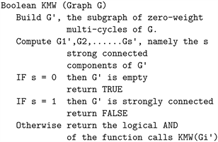
From the above pseudo-code, we conclude that the graph G, as well as the system of uniform recurrent equations it describes, is computable if and only if the function KMW (G) returns a value of TRUE. This is a recursive procedure that leads to the construction of a directed tree, whose vertices correspond to the original dependence graph and to the strongly connected components emerging from the graph decomposition procedure. The root of this tree structure is a vertex that corresponds to graph G. The number d of edges that constitute the path of maximum length in this tree structure is known as the depth of the decomposition. Note that this parameter can be defined in an alternative way, as the maximum number of calls to the recursive function KMW (G) generated by its first call (unless, of course, the graph is acyclic, in which case $d=0$ ). This depth d is considered as a measure of the parallelism described by the original graph G and is related to the maximum path length, as well as the minimum latency of the multi-dimensional affine scheduling function. It is proven that if the system of uniform recurrent equations described by the graph G is going to be characterized as computable, then the set of $d_{\upsilon }$ vectors $x_{\upsilon }^1\mathrm{,}{x}_{\upsilon }^2\mathrm{,}\cdots \mathrm{,}{x}_{\upsilon }^{d_{\upsilon }}$ generated during the execution of the algorithm for vertex $\upsilon$ , describing corresponding separating hyperplanes, is a linearly independent set of vectors, a property that always holds, for the set of the first $d_{\upsilon }-1$ vectors $x_{\upsilon }^1\mathrm{,}{x}_{\upsilon }^2\mathrm{,}\cdots \mathrm{,}{x}_{\upsilon }^{d_{\upsilon -1}}$ of this set. Therefore, the depth d of the decomposition is bounded by the value $n+1$ , where n is the dimension of the iteration space, or by the value n when the graph G is computable. This property allows the computation of an upper bound regarding the time complexity of the decomposition algorithm [27] .

Let us conclude this presentation, by noting that the sequence of vectors $x_{\upsilon }^1\mathrm{,}{x}_{\upsilon }^2\mathrm{,}\cdots \mathrm{,}{x}_{\upsilon }^{d_{\upsilon }}$ and the corresponding constants ${\rho }_{\upsilon }^1\mathrm{,}{\rho }_{\upsilon }^2\mathrm{,}\cdots \mathrm{,}{\rho }_{\upsilon }^{d_{\upsilon }}$ obtained from the above dual program, allows the definition of d-dimensional scheduling function $S\mathrm{<mo>\; :\; </mo>}V\times P\mapsto {\mathbb{Q}}^d$ as a mapping of the form:

$\left(\upsilon \mathrm{,}p\right)=\left(x_{\upsilon }^1+{\rho }_{\upsilon }^1\mathrm{,}{x}_{\upsilon }^2+{\rho }_{\upsilon }^2\mathrm{,}\cdots \mathrm{,}{x}_{\upsilon }^{d_{\upsilon }}+{\rho }_{\upsilon }^p\mathrm{,0,0,0},\cdots \mathrm{,0}\right)$

In the above expression, the zero values added to the end of the tuple are required to make this tuple, a set of d elements. Darte and Vivien [24] , prove that for every edge $e\in E$ and for every $p\in R$ , this function satisfies the property $S\left(x_e\mathrm{,}p\right)\gg S\left(y_e\mathrm{,}p-w\left(e\right)\right)$ and thus is indeed a valid d-dimensional scheduling function. The above is always valid for strongly connected graphs. On the other hand, if the graph is not strongly connected, then: a) the strongly connected components of the graph are identified, b) the multi-dimensional scheduling function is constructed separately for each connected, and c) each one of these components, is scheduled with respect to the other, using topological sort on an acyclic graph, consisting of these strongly connected components. It turns out that if the dimension of this multi-dimensional scheduling function, is equal to d, then the latency caused by this function is characterized by a complexity $O\left(N^d\right)$ , where N is a measure of the iteration space. On the other hand, the maximum dependency path length in the EDG graph, which gives a lower bound of the sequential nature of the system and consequently, an upper bound of the degree of parallelism, has a complexity of $\Omega \left(N^d\right)$ . This implies that the system of uniform recurrent equations described by the graph G, contains a degree of parallelism equal to $\left(n-d\right)$ , that can be extracted in the appropriate way.

11. The Systems of Uniform Recurrent Equations and Nested Loops

Is there any relationship between systems of recurrent equations and nested loops? This question stems in a natural way from the fact, that both these computational structures share a lot of common concepts and definitions, such as the concepts of iteration space and iteration vectors, and furthermore, they are involved to common procedures, such as the identification of the optimal scheduling functions. In fact, the multiple nested loops can be considered as special cases of systems of recurrent equations, and therefore, what we have said in the previous sections, can also be used to describe nested loops, too, even though some concepts are defined and used in different ways.

In particular, let us consider a multiple nested loop of depth $d=n$ , in which the innermost loop contains $m+1$ statements. In this case, a set of m dependency vectors can be defined that allows the description of the system via an equation in the form:

$u\left(j\right)=g_j\left[u\left(j-d_1\right)\mathrm{,}u\left(j-d_2\right)\mathrm{,}\cdots \mathrm{,}u\left(j-d_m\right)\right]$

where: a) $j$ is a vector of the iteration space $\mathcal{J}$ with $n>0$ integer components, b) $g_j$ is the computation associated with the iteration vector $j$ which should be completed in a time interval of a duration equal to unity, c) $\upsilon \left(j\right)$ is the result of the computation $g_j$ and d) $d_i\in {\mathbb{Z}}^n$ $\left(1\le i\le m\right)$ are constant integer vectors of length n, describing the uniform dependencies, that jointly define the dependence matrix $D$ . It is not difficult to see, that such a description of the dependencies, leads to equations similar to the ones describing a system of uniform recursive equations, and as Shang and Fortes point out [17] , this class of uniform dependencies can be seen as an extension of the class of computations described by uniform recurrent equations. In the case of nested loops, it is possible to compute the values of different functions at different points in the index set, although there is still the requirement of performing these computations in unit time. In the above equations, for each point $j\in \mathcal{J}$ , the points $j-d_i$ also belong to the iteration space $\mathcal{J}$ , while the dependence vectors are constant and independent of $j$ .

The most important difference between nested loops and systems of uniform recursive equations is the execution order of the required iterations. In particular, in nested loops, this order is determined, by the so-called lexicographic order, which is dictated by the fact that for each iteration of the outer loops, all iterations of the inner loops are executed one after the other. Although in nested loops, all kinds of dependencies can occur, such as flow dependencies, output dependencies, as well as anti-dependencies, however, the dependence vectors should always be lexicographically positive. Consequently, the Extended Dependence Graph (EDG) for the case of a perfect nested loop with uniform dependencies, will always be an acyclic graph, while the corresponding Reduced Dependence Graph (RDG), does not contain zero-weight cycles.

On the other hand, in the systems of uniform recursive equations, the situation is quite different. Now, there is no such type of lexicographic order with respect to the execution of iterations, since any computation can be performed once the values of all required quantities have already been computed and are available for use. This means that all the dependencies are flow dependencies, and there is no requirement for the dependence vectors to be lexicographically positive vector. The occurrence of zero-weight cycles in the dependence graph of such a system is now possible, and thus, unlike a perfect nested loop, whose execution is always guaranteed, provided that the above conditions are met, a system of uniform recurrent equations, may or may not be computable, depending of the detection of zero-weight cycles in the dependence graph.

Finally, as we said before, a computational structure emerged from a nested loop is acyclic, meaning that the validity of the condition $a_0{d}_0+a_1{d}_1+\cdots +a_k{d}_k=0$ , where $a_1\mathrm{,}{a}_2\mathrm{,}\cdots \mathrm{,}{a}_{k-1}$ are non-negative integers and $d_0\mathrm{,}{d}_1\mathrm{,}\cdots \mathrm{,}{d}_{k-1}$ are dependence vectors, implies that $a_1=a_2=\cdots =a_{k-1}=0$ . This property is a natural consequence of the fact that if the structure is not acyclic but instead cyclic, meaning that there are mutual dependencies between the data sets, deadlock may be inserted in the picture. An exception to this rule is the case in which, some of the above vectors are not actual vectors, but instead, virtual dependence vectors, meaning that they are associated with dependencies, that do not involve computations, but only data transmission between iterations. In the latter case, because no computation is involved, this transmission can be done immediately, without delay, and therefore, generally speaking, the appearance of deadlocks is not possible. It is important to note, that the requirement for a structure to be acyclic, allows us to define the granularity of the computational work and enables the possibility of parallelization via the mechanism of pipelining.

Of course, despite the above differences, the high degree of similarity between these computational structures, allows us to study them, using the same techniques, and more specifically, to identify scheduling functions and to perform data and iteration partitioning. It is not difficult to see, that the processes of scheduling and partitioning, which are inextricably linked to the parallelization of a nested loop, have their origin in this connection between nested loops and systems of uniform recurrent equations.

12. Conclusion

Although it has been 57 long years since the publication of the paper of Karp, Miller and Winograd, its importance is still not disputed by anyone, since the issues of computability and the schedulability defined in this work, are characteristic of every algorithm and every computational structure in our days. To conclude this brief presentation, let us mention hor historical reasons, that one of the most important applications of this theory, which appeared 15 years after the publication of KMW, and more specifically in the early 1980s, was the design of systolic arrays [28] .

NOTES

¹Here, the subscript k is omitted because there is a single equation and hence a single function $\alpha \left(p\right)$ .

Conflicts of Interest

The author declares no conflicts of interest regarding the publication of this paper.

References

[1]	Karp, R.M., Miller, R.E. and Winograd, S. (1967) The Organization of Computations for Uniform Recurrence Equations. Journal of the ACM, 14, 563-590. https://doi.org/10.1145/321406.321418
[2]	Darte, A. (2010) Understanding Loops: The Influence of the Decomposition of Karp, Miller, and Winograd. Eighth ACM/IEEE International Conference on Formal Methods and Models for Codesign (MEMOCODE 2010), Grenoble, 26-28 July 2010, 139-148. https://doi.org/10.1109/MEMCOD.2010.5558638
[3]	Lamport, L. (1974) The Parallel Execution of DO Loops. Communications of the ACM, 17, 83-93. https://doi.org/10.1145/360827.360844
[4]	Moldovan, D.I. (1982) On the Analysis and Synthesis of VLSI Algorithms. IEEE Transactions on Computers, 31, 1121-1126. https://doi.org/10.1109/TC.1982.1675929
[5]	Quinton, P. (1984) Automatic Synthesis of Systolic Arrays from Uniform Recurrent Equations. ACM SIGARCH Computer Architecture News, 12, 208-214. https://doi.org/10.1145/773453.808184
[6]	Allen, J.R. and Kennedy, K. (1987) Automatic Translation of FORTRAN Programs to Vector Form. ACM Transactions on Programming Languages and Systems, 9, 491-542. https://doi.org/10.1145/29873.29875
[7]	Chapra, S.C. and Canale, R.P. (2015) Numerical Methods for Engineers. 7th Edition, McGraw-Hill, New York, 855-856.
[8]	Tanenbaum, A. and Bos, E. (2014) Modern Operating Systems. 4th Edition, Pearson, London.
[9]	Feautrier, P. (1992) Some Efficient Solutions to the Affine Scheduling Problem. I. One-Dimensional Time. International Journal of Parallel Programming, 21, 313-347. https://doi.org/10.1007/BF01407835
[10]	Taha, H. (2022) Operations Research: An Introduction. 11th Edition, Pearson, London.
[11]	Quinton, P. and Van Dongen, V. (1989) The Mapping of Linear Recurrence Equations on Regular Arrays. Journal of VLSI Signal Processing Systems, 1, 95-113. https://doi.org/10.1007/BF02477176
[12]	Rajopadhye, S.V. and Fujimoto, R.M. (1990) Synthesizing Systolic Arrays from Recurrence Equations. Parallel Computing, 14, 63-189. https://doi.org/10.1016/0167-8191(90)90105-I
[13]	Feautrier, P. (1992) Some Efficient Solutions to the Affine Scheduling Problem. Part II. Multi-Dimensional Time. International Journal of Parallel Programming, 21, 389-420. https://doi.org/10.1007/BF01379404
[14]	Darte, A. and Robert, Y. (1995) Affine-by-Statement Scheduling of Uniform and Affine Loop Nests over Parametric Domains. Journal of Parallel and Distributed Computing, 29, 43-59. https://doi.org/10.1006/jpdc.1995.1105
[15]	Schrijver, A. (1986) Theory of Integer and Linear Programming. John Wiley & Sons, Hoboken.
[16]	Chernikova, N.V. (1965) Algorithm for Finding a General Formula for the Non-Negative Solutions of a System of Linear Inequalities. USSR Computational Mathematics and Mathematical Physics, 5, 228-233. https://doi.org/10.1016/0041-5553(65)90045-5
[17]	Shang, W. and Fortes, J.A.B. (1991) Time Optimal Linear Schedules for Alforithms with Uniform Dependencies. IEEE Transactions on Computers, 40, 723-742. https://doi.org/10.1109/12.90251
[18]	Feautrier, P. (1989) Asymptotically Efficient Algorithms for Parallel Architectures. In: Cosnard, M. and Girault, C., Eds., Decentralized Systems, IFIP WG 10.3, North-Holland, 273-284.
[19]	Berge, C. (1962) The Theory of Graphs and Its Applications. Wiley, New York.
[20]	Cohen, E. and Megiddo, N. (1989) Strongly Polynomial-Time and NC Algorithms for Detecting Cycles in Dynamic Graphs. Prodceedings of 21st Annual ACM Symposium on Theory of Computing, Seattle, 14-17 May 1989, 523-534. https://doi.org/10.1145/73007.73057
[21]	Darte, A., Khachiyan, L. and Robert, Y. (1991) Linear Scheduling Is Nearly Optimal. Parallel Processing Letters, 1, 73-81. https://doi.org/10.1142/S0129626491000021
[22]	Dantzig, G.B. (1963) Linear Programming and Extensions. Princeton University Press, Princeton. https://doi.org/10.7249/R366
[23]	Rao, S.K. and Kailath, T. (1988) Regular Iterative Algorithms and Their Implementation on Processor Arrays. Proceedings of the IEEE, 76, 259-269. https://doi.org/10.1109/5.4402
[24]	Darte, A. and Vivien, F. (1995) Revisiting the Decomposition of Karp, Miller and Winograd. Proceedings of the International Conference on Application Specific Array Processors, Strasbourg, 24-26 July 1995, 13-25. https://doi.org/10.1109/ASAP.1995.522901
[25]	Bellman, R. (1958) On a Routing Problem. Quarterly of Applied Mathematics, 16, 87-90. https://doi.org/10.1090/qam/102435
[26]	Ford Jr., L.R. (1956) Network Flow Theory. RAND Corporation, Santa Monica, CA.
[27]	Darte, A. and Vivien, F. (1994) Automatic Parallelization Based on Multidimensional Scheduling. Technical Report 94-24, Laboratoire de 1’Informatique du Parallélisme, Ecole Normale Supérieure de Lyon, Lyon.
[28]	Quinton, P. (1983) The Systematic Design of Systolic Arrays. Rapports de Recherche, No. 216, Centre de Rennes, Institut de Researche en Informatiwue et den Automatique, Bruz.